1. Introduction

Nowadays, image analysis and object detection on images play a key role in many fields, including industry, robotics, and medical diagnosis [1-3]. The use of digital technologies is considered one of the approaches that can help improve the quality of healthcare services and the experience of patients, physicians, and other service recipients [4]. Among e-health services, telemedicine [5] and mobile health based services are becoming increasingly popular. In 2016, IBM researchers estimated that 90% of all medical data were images [6]. Accordingly, a huge number of methods have been developed to analyze medical images, which are well described in the literature [7].

Methods of analyzing medical data using machine learning algorithms are becoming widespread [8]. In particular, they are used to solve the problems of classifying the types of brain and lung lesions and making a diagnosis [9 -11]. However, machine learning algorithms are often developed and tested on high-quality data, such as MRI and CT images, presented as 3D or 4D images with low noise and high spatial resolution. At the same time, visualization and analysis of such data are rather laborious and also requires the use of specialized software that allows the user to upload and then view data in specific formats (NIfTI, DICOM). In real life, for quick information exchange about the condition of patients, as well as for telemedicine consulting, medical specialists frequently take photos of the computer screen on which the result of the MRI scans is displayed. Telemedicine today is just beginning to gain popularity in the Russian market. During the COVID-19 pandemic, the need for remote transmission of medical data has emphasized the importance of developing reliable algorithms to provide medical care at a distance [11]. One of the major advantages of telemedicine is the saving of time and financial resources, and allowing consultations with subspecialty physicians without them having to move [12]. Also, when using telemedicine, patients have the opportunity to remotely transmit data about their health status, including photos taken with a smartphone camera. However, in this case, the quality of images deteriorates and additional noise appears on them, which can lead to unstable operation of standard methods of image analysis [13]. In addition, we note that the developed algorithms should not be labor-intensive in computations in order to be suitable for mobile use.

The purpose of the present study is to compare the performance of different algorithms in the task of detecting brain structures on MRI images taken by a smartphone from the monitor screen.  The criteria for comparison will be the accuracy of object detection in the image, the amount of memory occupied by the model, and the number of elementary operations carried out by the model.

In this paper, we analyzed and compared four approaches to solving the problem of object detection in an image: the morphometric approach [14], the Viola-Jones algorithm [15, 16] and two neural network models: YOLOv8 [17] and EfficientDet [18]. The morphometric approach is one of the common medical image preprocessing methods for machine learning [19], which allows the user to find objects in an image using standard OpenCV library functions without using deep learning algorithms. However, it remains unknown how robust this algorithm is when dealing with poor quality images. The Viola-Jones algorithm is also a common and long-used method for automatic object recognition [20,21], so it is particularly interesting to compare it with the most popular modern deep learning algorithms such as YOLOv8 and EfficientDet. The above approaches were analyzed, taking into account their advantages and limitations in the context of the task presented.

2. Description and formalization of initial data

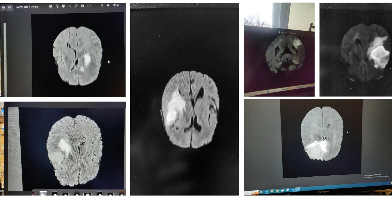
A special set of images was prepared for the training and testing of the considered algorithms. The open clinical dataset BraTS-19 [22-24] was taken as a basis. This database contains extensive routine clinical preoperative MRI images of glioblastoma and brain glioma. Among the different imaging modalities presented in NIfTI (.nii) file format, images recorded using FLAIR sequences were selected because they are the most widely used in the context of malignant glioblastoma detection. From the selected 3D images, several cross-sections were visualized, which were then converted into PNG images using the NiBabel library [25] and photographed using the cameras of different smartphones (Samsung Galaxy S10e, 12 MP; Samsung Galaxy A50, 25 MP; Redmi Note 10 pro, 108 MP). A total of 631 images were prepared. Examples of the resulting images are presented in Fig.1.

 

Fig. 1. Examples from the training set

 

It is worth noting that the images may contain a variety of extraneous objects: desktop icons, glare, reflections, and other noise — in order to simulate as closely as possible the images that may occur during real clinical practice. All images were then manually labeled by the authors using the Roboflow tool [26].

We introduce the concept of a bounding box, which is a rectangle containing the objects of interest to the analytical model. The boundaries of such a box are defined by two coordinates: upper left and lower right corners. Bounding boxes are widely used in detection tasks due to a clear formalization of the description of the object location in the image. This allows accurate detection of object boundaries and the use of these frames in various tasks related to image analysis.

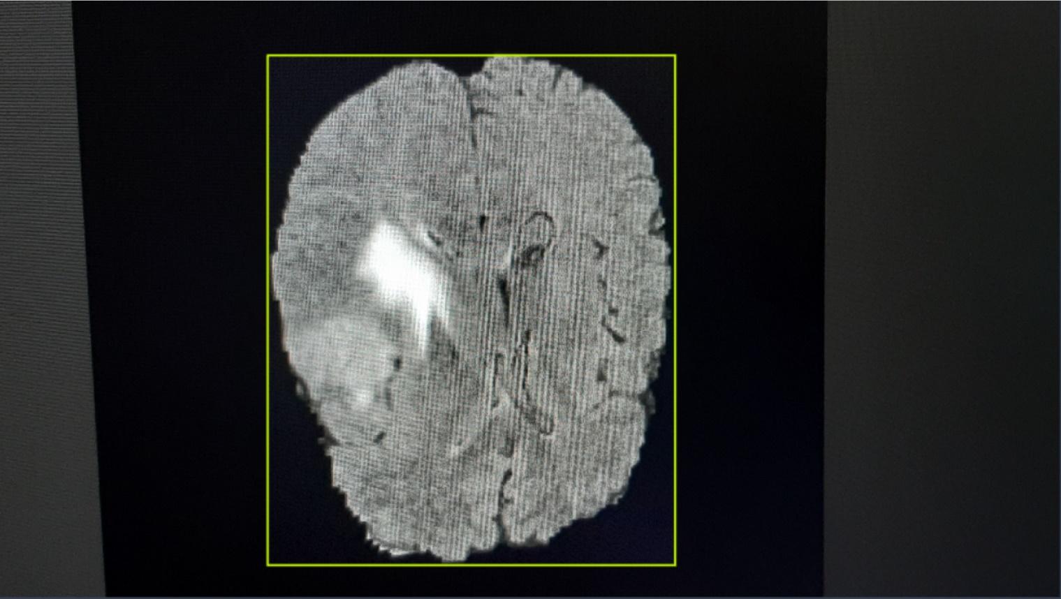
Thus, the contours of the brain were surrounded by bounding boxes and classified as the class “brains”, the other objects in the image were not classified in any way.  An example of a labeled image is shown in Fig. 2.

 

Fig. 2. Example of an annotated image

 

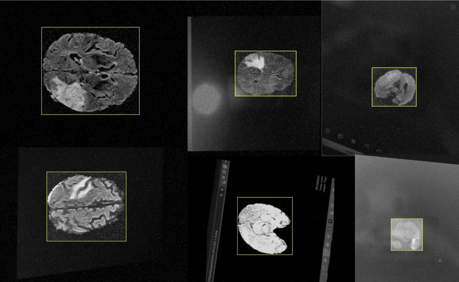
Since the training efficiency of the neural network depends on the amount of data and becomes more robust when noise is present in part of the training dataset [19], image augmentation techniques, such as 90° rotation, adding points to the image, image blurring, specular reflection and perspective distortion were used to broaden the sample. Examples of images with the listed augmentations are presented in Fig. 3.

 

Fig. 3. Examples of augmented images

 

After augmentation, a set of 1038 images was obtained. They were divided into training and test samples in the proportion of 8:2. As a result, 814 images were included in the training sample and 224 images in the test sample.

3. Methodology

The study compares four approaches for detecting objects in an image: the use of standard OpenCV library methods (such as applying morphological transformations to a binarized image), called the morphometric approach, the use of the Viola-Jones algorithm, and two deep learning methods: neural networks with the YOLOv8 architecture and with the EfficientDet architecture. Each of the four approaches is described in detail below.

3.1. Morphometrical approach

A number of works related to medical image processing [14, 27] use some functions from the OpenCV library to process an image or to prepare an image for use in training a neural network.

OpenCV (Open Source Computer Vision Library) [28] is an open source library for working with computer vision algorithms, machine learning and image processing. This library is implemented in C/C++, but it is also developed for Python, Java, Matlab and other languages. In this paper, we used the Python version of the library.

We created a 6-step algorithm to extract the outline of the largest object in the image and draw a bounding box around it, based on the information described in the above sources.

The initial dataset contains images with one large object — the contour of the brain and a background. In this case, the background of the image is black, but in addition to it, other objects described above (desktop icons, screen frame, etc.) may also be on the photo. The contours of the brain in the image must be the largest contour. To find it, we propose to use the following algorithm:

1. Convert an image to grayscale.

2. Apply binarization to the obtained image. To find the threshold of binarization we use Otsu's algorithm [29]. Thus, the pixels belonging to the lighter region — the contour of the brain — should fall into the “useful” class, while the rest fall into the “background” class.

3. Apply the morphological closing operation to a binarized image with a 3×3 kernel. This operation helps to eliminate small holes or dots in objects and merge them.

4. Find all external contours in the transformed image [30]. After applying the previous operations, the main object became absolutely white, and the background became black. In this case, the contours will be understood as curves connecting continuous points (along the boundary) having the same color and brightness, i.e., the objects with the highest brightness in the image will be detected.

5. Among the found contours, choose the contour bounding the figure of maximum area. To do this, calculate the areas of all found contours using the Green- Ostrogradsky formula:

where functions are determined in space D, restricted by a certain curve C and have partial derivatives .

6. Draw a bounding box around the identified contour.

This algorithm gives us the coordinates of the rectangles, presumably bounding the brain in the image.

3.2. Viola-Jones Algorithm

The Viola-Jones algorithm is one of the first object detection methods [20] that became widely used. However, this method has recently been losing popularity due to the emergence of new machine learning methods that demonstrate higher accuracy in recognizing the original objects [21]. A significant advantage of the method is that it demonstrates a low computational load on the system [31], which can be very useful if it is used as part of a more complex image processing system.

This method is based on an integral image representation, which can efficiently compute the total brightness of pixels in rectangular regions of an image by applying preprocessing [15,16]. This significantly reduces the computational complexity of the operations and allows fast feature computation at different scales and different object positions in the image.

The present algorithm incorporates the adaptive boosting algorithm [20], which is a learning method with successive tuning of weak classifiers (simple models that do not have high prediction accuracy) based on the errors of the previous classifier. In this way, the classification accuracy is gradually improved. Combining a set of weak classifiers together with a specific weight for each of them results in a stronger model. Typically, the weight for each weak classifier is determined iteratively during the adaptive boosting training process, where the weights are updated based on how well the model handles certain data samples.

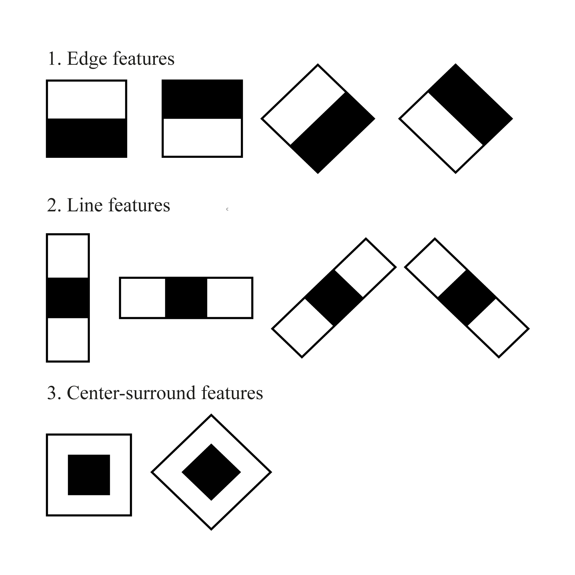
One of the key components of the Viola-Jones algorithm, in addition to those listed above, is the use of Haar features to find the object being searched for. Haar features are rectangular regions of different sizes such as horizontal, vertical and diagonal stripes. These features are used to calculate various image features on the basis of which the object will be classified. The combinations of features form the cascading structure of the classifier. A visualization of the Haar features is shown in Fig. 4.

 

Fig. 4. Haar features

 

The overall cascade structure obtained by the Viola-Jones method is called Haar's Cascade. The cascade is widely used to detect objects such as faces, eyes, cars, etc. It is also capable of finding the movements of the searched object in the video and tracking them.

Haar’s Cascade is the most commonly used of all the object recognition methods considered in this paper. Nonetheless, a significant drawback of this algorithm is that it is arduous on the quantity of images in the training sample owing to the utilization of bouncing in training [17]. It is also arduous on the brightness of the images due to the utilization of a brightness-aware method in the training algorithm.

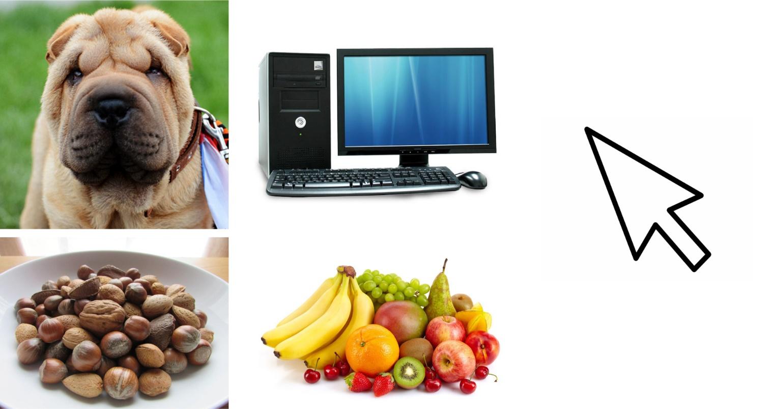
In this work, 814 positive images (407 original + 407 augmented) containing an object of the class “brains” and 1,000 negative images without objects of the desired class were used in training the cascade. Negative images included snapshots of desktop screens, mouse cursors, etc. — in order to reduce the sensitivity of the cascade response to the presence of these objects in the positive sample, as well as images of irrelevant objects: animals, fruits, vegetables, and nuts (Fig. 5).

 

Fig.5. Some images from negative sampling

 

In this study, a cascade was created using the Cascade Trainer GUI program, which is a graphical interface for applying algorithms from the OpenCV library.

The cascade was trained for 20 epochs, after which a required false alarm rate of the classifier of 10% was achieved. At the same time, the acceptance ratio of the classifier was 0.0002, which means that the classifier is accurate enough and the model has not yet been overtrained. Thus, the creation of the cascade took 1,442 minutes. Training was performed on an AMD Ryzen 5 processor, 4 performance cores, frequency 2.10 GHz.

3.3. YOLOv8

YOLO (You Only Look Once) is a family of models for solving the multi-class detection problem. YOLO models are widely used for object detection in medical image processing [32]. The multi-class detection task in deep learning is conventionally composed of two subtasks. The first one is finding candidate bounding boxes, i.e., such bounding boxes in the image, within which at least one of the searched objects is most likely to be located. The second task is to classify the identified candidate bounding boxes by selecting the class with the highest calculated probability of being located within a given bounding box.

Earlier architectures, such as R-CNN [33], Fast R-CNN [34] or Faster R-CNN [35] solved the above tasks in two separate steps, whereas YOLO solves both tasks in a single step, which is reflected in the name of the method.

The basic version of the YOLO model [17] is a convolutional neural network architecture from the “Darknet” family [36] and two fully connected layers. The basic version of YOLO uses the “Darknet-17” architecture. Note that “Darknet” in this case refers to the architecture and not to a deep learning framework with a similar name.

YOLO inputs an image and outputs vectors for each of the remaining bounding boxes after a “Non-maximum suppression” procedure, which leaves the most relevant one out of several very similar bounding boxes, excluding the rest from the final detection.

Since 2015, the YOLO family has seen various “newcomers” [32]. The most recent of these at the time of writing is the eighth version of YOLO, namely YOLOv8. In this model, object detection checkpoints are pre-trained on the MS-COCO dataset [37], and image classification models are pre-trained on the ImageNet set [38], allowing for a more stable multi-class detection quality.

Ultralytics [39], the official library of YOLOv8 developers, was used to run the model. The pre-trained model was further trained on a dataset created by the authors using stochastic gradient descent (AdamW algorithm with a learning rate equal to 0.002 and momentum equal to 0.9) with the selection of hyperparameters after each epoch on a validation sample of 100 images. 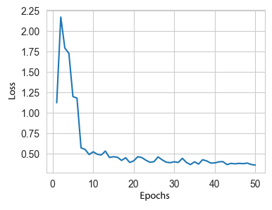Data for the validation sample were randomly selected from the training sample. The model was trained for 50 epochs, after which the value of the error function stopped decreasing and there was a danger of over-fitting. The process of changing the value of the loss function during 50 epochs is illustrated in Fig. 6.

 

Fig. 6. Graph of convergence of training results of the YOLOv8 model

 

A threshold value of 0.7 was placed on the probability of finding an object of the class “brains”. The value was selected as a hyperparameter in order to achieve the highest average Intersection over Union (IoU) metric.

YOLOv8 was trained in the Google Colaboratory interactive environment using a T4 GPU, with a training time of 25 minutes.

3.4. EfficientDet

EfficientDet (D0-D7) [18] are models from the innovative class of neural network models EfficientNet [40], designed for object detection in images. This model is based on the EfficientNet architecture, on top of which a layer working with the Bidirectional Feature Pyramid Network (BiFPN) is added, followed by a classifier network for generating object class predictions and a block network for bounding box prediction. Focusing on mobile and embedded applications, TensorFlow Lite (TF Lite) [41] developed the EfficientDet-lite family of object detection models using convolutional architectures standard to this family of models, but formatted for small model size and fast output. However, their performance is slightly inferior to the original EfficientDet family counterpart. This study used the EfficientDet-lite (lite0) object detection model pre-trained on the MS-COCO 2017 dataset [37]. Based on the results of the model's comparison, the authors plan to integrate the selected approach into a large automatic diagnosis system. Therefore, the speed of operation and the small size of the model interested us from a research perspective, and this model was chosen. The number of output classes of the model was changed (the MS-COCO 2017 dataset contains 91 classes of objects, and in the task at hand, the model should detect only one class - “brains”), and the threshold value of the probability of detecting an object in an image was set to 0.7, similar to the YOLOv8 model described above. This was done for correctness of comparison of the final results. 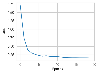The model was pre-trained using the error back propagation method using a stochastic gradient descent with an inertia of 0.9, an initial step of 2*10^-2, and a cosine attenuation multiplier of 4*10e-5. The model was pre-trained for 20 epochs, after which the loss function stopped decreasing. This process is illustrated in Fig. 7.

 

Fig. 7. Graph of convergence of training results of EfficientDet-lite (lite0) model

 

The model was trained on a PC with an AMD Ryzen 3 processor, 4 performance cores, frequency 2.6 GHz. The training took 162 minutes on the described computer.

3.5. Quality metrics

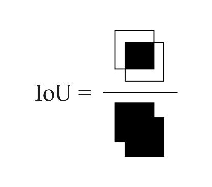
For object detection tasks in an image, the choice of a quality metric that indicates how well the model solves the problem is also important. The IoU metric is widely used to evaluate the quality of model performance in segmentation and object detection tasks in computer vision. IoU has a simple and interpretable formula that reflects the ratio between the area of the intersection region of the rectangles bounding the true and predicted objects and their total area (Fig.8).

 

Fig. 8. Graphic interpretation of the IoU-metric

 

In this case, it is easy to interpret how well the model detects objects. To compare the performance of different methods, the average value of this metric on the test sample was calculated. In Section 4, Table 1 shows not only the mean values of the metric, but also the maximum and minimum over the sample, in column 2. Since, in this study, only one class of objects is searched for in the image and the result is a single bounding box, the use of this metric is more appropriate than using common metrics such as average precision (AP) and mean average precision (mAP).

In addition to the IoU metric, the number of elementary operations that were required to run the algorithms on the test sample was measured as a measure of algorithm performance. This metric is independent of the device on which the model is run. A standard python language module, cProfile, was used to analyze program performance and calculate the number of elementary operations.

4. Results

The results of the computational experiments are described in Table 1.

Table 1 Comparison of algorithms

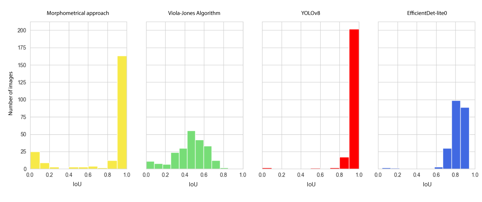
The YOLOv8 model demonstrated the best average quality of object detection on the test sample. However, it was found that the performance of all considered models strongly depended on the presence of noise in the image. For a more detailed analysis of the algorithms' performance quality, histograms of the distribution of the object detection quality on the image were plotted (Fig.9).

 

Fig. 9.  Histograms of the distribution of IoUs' values based on the results of object detection provided by different models

 

For example, for images with little noise and sufficient contrast between the object (brain) and the background, the morphometric algorithm detected the object with an accuracy of up to 99.9%. However, the presence of strong noise in the image reduced its accuracy to almost 0%. It can be concluded that this algorithm processed most of the images with very high accuracy. Machine learning algorithms proved to be more resistant to image noise and demonstrated stable results for almost the entire sample. Nevertheless, the factor of noise presence was significant for them as well. 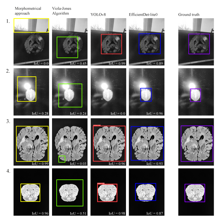The IoU distribution for the YOLOv8 model was the most skewed to the right, i.e., YOLOv8 almost always shows a score of 0.8 or higher, except for one photo (Fig. 8) when the model is unable to find an object. In this image, a strong noise is created by the flash from the camera, which obviously biases the model. The EfficientDet model successfully detected brain contours in all images, even in the presence of strong noise. However, the average quality of object detection in the image of this model is worse compared to YOLOv8, which is due to the lower accuracy of finding the bounding box. The Viola-Jones algorithm on the presented sample showed the worst result in terms of IoU -metrics, but we can note a certain stability in its work: it can detect the brain on images of any quality.

Fig.8 shows examples of algorithm results on good quality images and on images with a lot of noise.

 

Fig. 10. Results of algorithms' work on images with different noise levels. 1, 2: highly noisy images, 3, 4: high-quality images

 

The study also revealed that the Viola-Jones algorithm is the least costly in terms of the number of operations, and it occupies the least memory space. The morphometric approach is also very close to Viola-Jones in those parameters. However, there are serious obstacles for using both of these methods: in the case of the Viola-Jones algorithm: very low accuracy, and in the case of morphometric approach — instability of the algorithm in the presence of strong noises in the image.

5. Conclusion

In this paper, four methods of brain detection in a computer screen MRI image have been compared. All tested approaches demonstrate a quite high average performance of object detection in the image. The YOLOv8 model demonstrated the highest average IoU object detection performance, however, this model is massive in terms of computer memory and its performance is sensitive to noise in the image. The EfficientDet-lite0 model demonstrated a slightly lower quality of object recognition on average, but proved to be more robust to noise. Another advantage of this model is its light weight. The volume of the model is important for its further incorporation in more complex neural network diagnostic systems, for which object detection will be only the first step. The classical morphometric approach to the detection of a large object in the image has also demonstrated high results, but it cannot be used to solve the problem because this algorithm recognizes the largest light area in the image. In the case of image illumination or a random light object in the frame, it works incorrectly. The Viola-Jones algorithm poorly coped with the task of detecting brain structures on the MRI image and is not recommended for use within the described task.

6. Acknowledgements

The study was supported by the Academic Fund Program at HSE University (grant No 23-00-026 “Development of automatic approaches to determine the etiology of cryptogenic stroke for the purpose of preventing secondary acute cerebrovascular accidents”).

The authors would like to thank Sofia Petrovna Kulikova, Head of the Center for Cognitive Neuroscience, National Research University Higher School of Economics, Perm, for her help in preparing the article.

Literature

1. Song S. et al. EfficientDet for fabric defect detection based on edge computing //Journal of Engineered Fibers and Fabrics, Vol. 16, 2021 (https://doi.org/10.1177/15589250211008346).

2. Afif M. et al. An evaluation of EfficientDet for object detection used for indoor robots assistance navigation //Journal of Real-Time Image Processing, Vol. 19 (3), 2022, pp. 651-661 (http://dx.doi.org/10.1007/s11554-022-01212-4).

3. Mercaldo F. et al. Object Detection for Brain Cancer Detection and Localization //Applied Sciences, Vol. 13 (16), 2023, pp. 9158 (http://dx.doi.org/10.3390/app13169158).

4. Moghaddasi H. et al., E-health: a global approach with extensive semantic variation //Journal of medical systems, Vol. 36, 2012, pp. 3173-3176 (http://dx.doi.org/10.1007/s10916-011-9805-z).

5. Pol P., Deshpande A.M. Telemedicine mobile system //2016 Conference on Advances in Signal Processing (CASP), IEEE, 2016, pp. 484-487 (http://dx.doi.org/10.1109/CASP.2016.7746220).

6. Landi H. IBM Unveils Watson-Powered Imaging Solutions at RSNA, òRSNA, 2016. Accessed: November, 29st, 2023. [Online]. Available: https://www.hcinnovationgroup.com/populationhealth-management/news/13027814/ibm-unveilswatsonpowered-imaging-solutions-at-rsna

7. Íåäçüâåäü À.Ì., Àáëàìåéêî Ñ. Â. Àíàëèç èçîáðàæåíèé äëÿ ðåøåíèÿ çàäà÷ ìåäèöèíñêîé äèàãíîñòèêè, Ìèíñê : ÎÈÏÈ ÍÀÍ Áåëàðóñè, 2012, Ñ.240 (ISBN 978-985-6744-75-7).

8. Papp L. et al. Personalizing medicine through hybrid imaging and medical big data analysis //Frontiers in Physics, Vol. 6, 2018, pp. 51 (http://dx.doi.org/10.3389/fphy.2018.00051).

9. Kumar S., Pilania U., Nandal N. A systematic study of artificial intelligence-based methods for detecting brain tumors // Èíôîðìàòèêà è àâòîìàòèçàöèÿ, Vol. 22 (3), 2023, pp. 541-575 (http://dx.doi.org/10.15622/ia.22.3.3).

10. Krishnapriya S., Karuna Y. Pre-trained deep learning models for brain MRI image classification //Frontiers in Human Neuroscience, Vol. 17, 2023, pp. 1150120 (http://dx.doi.org/10.3389/fnhum.2023.1150120).

11. Moreira L.P. Automated Medical Device Display Reading Using Deep Learning Object Detection // arXiv preprint arXiv:2210.01325, 2022 (https://doi.org/10.48550/arXiv.2210.01325).

12. Êîçëîâà À. Ñ., Òàðàñêèí Ä. Ñ. Òåíäåíöèè ðàçâèòèÿ òåëåìåäèöèíû è åå âëèÿíèå íà ñòðàõîâîé ðûíîê Ðîññèè //Ïðîìûøëåííîñòü: ýêîíîìèêà, óïðàâëåíèå, òåõíîëîãèè, 2018, Ò.2 (71), Ñ.144-148.

13. Mabotuwana T. et al. Detecting technical image quality in radiology reports //AMIA Annual Symposium Proceedings, American Medical Informatics Association, Vol. 2018, 2018, pp. 780.

14. Widodo C.E., Adi K., Gernowo R. Medical image processing using python and open cv //Journal of Physics: Conference Series, IOP Publishing, Vol. 1524 (1), 2020, pp. 012003 (http://dx.doi.org/10.1088/1742-6596/1524/1/012003).

15. Viola P., Jones M.J. Robust real-time face detection //International journal of computer vision, Vol. 57, 2004, pp. 137-154 (https://doi.org/10.1023/B:VISI.0000013087.49260.fb).

16. Freund Y., Schapire R., Abe N. A short introduction to boosting //Journal-Japanese Society For Artificial Intelligence, Vol. 14(771-780), 1999, pp. 1612 (https://doi.org/10.4236/jamp.2021.911186).

17. Redmon J. et al. You only look once: Unified, real-time object detection //Proceedings of the IEEE conference on computer vision and pattern recognition, 2016, pp. 779-788 (http://dx.doi.org/10.1109/CVPR.2016.91).

18. Tan M., Pang R., Le Q.V. Efficientdet: Scalable and efficient object detection //Proceedings of the IEEE/CVF conference on computer vision and pattern recognition, 2020, pp. 10781-10790 (http://dx.doi.org/10.1109/CVPR42600.2020.01079).

19. Z. et al. Improving synthetic CT accuracy by combining the benefits of multiple normalized preprocesses //Journal of Applied Clinical Medical Physics, 2023, pp. e14004 (http://dx.doi.org/10.1002/acm2.14004).

20. Viola P., Jones M. Rapid object detection using a boosted cascade of simple features //Proceedings of the 2001 IEEE computer society conference on computer vision and pattern recognition. CVPR 2001, IEEE, Vol. 1 2001, pp. I-I (http://dx.doi.org/10.1109/CVPR.2001.990517).

21. Sanjay T., Priya W.D. Criminal Identification System to Improve Accuracy of Face Recognition using Innovative CNN in Comparison with HAAR Cascade //Journal of Pharmaceutical Negative Results, 2022, pp. 218-223.

22. Menze B. H. et al. The multimodal brain tumor image segmentation benchmark (BRATS) //IEEE transactions on medical imaging, Vol. 34 (10), 2014, pp. 1993-2024 (http://dx.doi.org/10.1109/TMI.2014.2377694).

23. Bakas S. et al. Advancing the cancer genome atlas glioma MRI collections with expert segmentation labels and radiomic features //Scientific data, Vol. 4 (1), 2017, pp. 1-13 (https://doi.org/10.1038/sdata.2017.117).

24. Bakas S. et al. Identifying the best machine learning algorithms for brain tumor segmentation, progression assessment, and overall survival prediction in the BRATS challenge // arXiv preprint arXiv:1811.02629, 2018 (https://doi.org/10.48550/arXiv.1811.02629).

25. Brett M. et al. Nipy/ nibabel:. 4.0.0, Zenodo, 17.06.2022, (http://doi.org/10.5281/zenodo.6658382).

26. Dwyer B. et al. Roboflow (version 1.0)[software]. 2022.  Accessed: November, 29st, 2023. [Online]. Available:  https://roboflow.com.

27. Yousif M.J. Enhancing The Accuracy of Image Classification Using Deep Learning and Preprocessing Methods //Artificial Intelligence & Robotics Development Journal, 2023 (http://dx.doi.org/10.52098/airdj.2023348).

28. Bradski G. et al. OpenCV //Dr. Dobb’s journal of software tools, Vol. 3 (2), 2000.

29. Otsu N. A threshold selection method from gray-level histograms //IEEE transactions on systems, man, and cybernetics, Vol. 9 (1), 1979, pp. 62-66 (https://doi.org/10.1109/TSMC.1979.4310076).

30. Suzuki S. et al. Topological structural analysis of digitized binary images by border following //Computer vision, graphics, and image processing, Vol. 30 (1), 1985, pp. 32-46 (https://doi.org/10.1016/0734-189X(85)90016-7).

31. Ãàíèåâ Ì.À. Ìåòîäû äåòåêöèè îáúåêòîâ äëÿ àíàëèçà //Àêòóàëüíûå èññëåäîâàíèÿ, Ò. 10, 2024, Ñ. 48.

32. Qureshi R. et al. A Comprehensive Systematic Review of YOLO for Medical Object Detection (2018 to 2023), 2023 (https://doi.org/10.36227/techrxiv.23681679.v1).

33. Girshick R. et al. Rich feature hierarchies for accurate object detection and semantic segmentation //Proceedings of the IEEE conference on computer vision and pattern recognition, 2014, pp. 580-587 (https://doi.org/10.1109/CVPR.2014.81).

34. Girshick R. Fast R-CNN //Proceedings of the IEEE international conference on computer vision, 2015, pp. 1440-1448 (https://doi.org/10.1109/ICCV.2015.169).

35. Ren S. et al. Faster R-CNN: Towards real-time object detection with region proposal networks //Advances in neural information processing systems, Vol. 28, 2015 (https://doi.org/10.48550/arXiv.1506.01497).

36. Weng L. Object Detection Part 4: Fast Detection Models // lilianweng.github.io, 2018. Accessed: October, 15st, 2023. [Online]. Available:  https://lilianweng.github.io/posts/2018-12-27-object-recognition-part-4/.

37. Lin T.Y. et al. Microsoft COCO: Common objects in context //Computer Vision–ECCV 2014: 13th European Conference, Zurich, Switzerland, September 6-12, 2014, Proceedings, Part V 13. – Springer International Publishing, 2014, pp. 740-755 (https://doi.org/10.1007/978-3-319-10602-1_48).

38. Deng J. et al. Imagenet : A large-scale hierarchical image database //2009 IEEE conference on computer vision and pattern recognition, IEEE, 2009, pp. 248-255. (https://doi.org/10.1109/CVPR.2009.5206848)

39. Jocher, G., Chaurasia, A., Qiu, J. (2023). Ultralytics YOLO (Version 8.0.0) [Computer software], Accessed: November, 10st, 2023. [Online]. Available: https://github.com/ultralytics/ultralytics

40. Tan M., Le Q. Efficientnet: Rethinking model scaling for convolutional neural networks//International conference on machine learning, PMLR, 2019, pp. 6105-6114. (https://doi.org/10.48550/arXiv.1905.11946)

41. Abadi M. et al. TensorFlow: Large-scale machine learning on heterogeneous systems, 2015 (https://doi.org/10.48550/arXiv.1603.04467).