Early computer-aided
design (CAD) systems primarily used two approaches to geometric representation:discrete point sets (point clouds) and boundary representation (B-rep) [1]. Due
to the limited computing power of the time, engineers primarily used B-rep to
model geometric objects in CAD. This preference determined the evolution of
geometric solid modeling tools, making constructive solid geometry (CSG) a key
paradigm.
Today, technological
advances have significantly increased computing power, allowing researchers to
efficiently process large-scale point clouds obtained, for example, by laser
scanning [2, 3]. At the same time, engineers have increasingly integrated voxel
models [4, 5], another discrete geometric representation method, into their
practice. Today, discrete geometric modeling competes with continuous methods
as a key tool in engineering design.
Each modeling
paradigm has unique advantages and has certain limitations. For example,
converting CSG trees into explicit B-rep structures with defined faces, edges,
and vertices for production and visualization is a significant computational
challenge [6]. These persistent limitations and the limitations of traditional
solid modeling tools have prompted researchers to explore alternative geometric
representations.
A parametric approach
represents solids as ordered sets of points defined by point computations [7].
These models are conceptually similar to parametric solids (or hyper patches
[8]). This method views solid models as spatial regions containing points, or
equivalently, as volumes filled with the trajectory of a moving point.
Engineers can parameterize this point motion in a variety of ways, thereby
preserving the flexibility of geometric modeling.
The mathematical
framework of point computations [9] formalizes these models by generating point
equations that combine coordinate vectors (points) and parametric functions.
These equations reflect not only the external shape and position of an object,
but also the internal structure of its spatial region. This dual capability
allows researchers to easily transform continuous representations (point
equations) into discrete models (point clouds or voxels) using vectorization.
The authors of
studies [10, 11, 12], successfully applied this approach to modeling complex
geometric objects. However, applying Boolean operations to point solid models
for constructing complex technical systems using CSG methods remains an open
problem.
In this paper, we
describe geometric and computational algorithms developed for implementing
Boolean operations on solid models represented by sets of points.
In addition to the
computational formulations presented in this work, we consider a parametric
interpretation of point-based solid representation and Boolean evaluation. This
interpretation provides a parametric framework for understanding how ordered
point sets, generated from bounded parameter domains, support pointwise Boolean
operations without explicit topological construction. This perspective
clarifies the relationship between analytic formulation and the computational
procedures described in the subsequent sections.
The main
contributions of this paper are as follows:
1. A parametric representation of geometric solids as ordered point
sets based on point-based calculus.
2. A pointwise computational method for performing Boolean operations
without explicit topological structures.
3. A GPU-based implementation enabling interactive visualization of
Boolean operations on point-based models.
4. A natural-illumination model for point-based geometry that
combines ambient and Lambertian shading with an intersection-priority mechanism
for visually emphasizing Boolean-operation regions.
Within point-based calculus, a system does not treat a solid as a
collection of explicitly stored geometric entities. Instead, it generates
geometry procedurally by evaluating a parametric mapping. Accordingly, a solid
exists not as a static data structure, but as a rule for constructing points
over a bounded parameter domain.
This shift in
representation has important conceptual implications. Geometry is no longer
understood as a set of predefined surfaces and volumes, but as the result of a
generative process. The geometric object is reproduced whenever the parameter
domain is evaluated, and its structure is implicitly encoded in the parametric
formulation itself.
Formally, a solid
 is defined as
|

|
(1)
|
where
 is a bounded parametric domain,
 is an analytic point-generation mapping,
and
 denotes the dimensionality of the parameter space.
This interpretation
is consistent with the principles of point-based calculus, where solids are
defined through parametric point-generation mappings rather than explicit
boundary elements [7, 9].
This formulation
establishes a direct correspondence between the parametric domain and the
resulting point set. The domain
 determines the extent and internal structure of the solid, while
the mapping
 defines its shape and spatial configuration. As a result, the
geometric model is represented as an ordered set of points, where ordering is
induced by the parameters rather than by topological adjacency or spatial
proximity.
Key properties of
parametric point-based solids
The parametric
definition above implies a number of fundamental properties that distinguish
point-based solids from boundary-based and implicit representations.
1. Procedural generation of geometry. Geometry is defined through a
generation process. Each point is computed independently by evaluating the
mapping
 ,
enabling flexible sampling strategies.
2. Unified representation of boundary and interior. No distinction is
made between surface and volume at the representation level. Boundary elements
arise as limiting cases of the parameter domain, while interior points are
obtained by allowing parameters to vary freely.
3. Absence of explicit topology. Topological entities such as faces,
edges, and vertices are not introduced explicitly. Connectivity is not stored
or reconstructed, eliminating topological inconsistencies common in
boundary-based models.
4. Ordered point structure. Each generated point is uniquely
associated with specific parameter values, which define its parametric identity
and enable consistent interpretation of geometric structures.
Constructive principles
of solid generation
In point-based
calculus, solid geometry may be constructed in a constructive manner by
extending lower-dimensional parametric entities into volumetric domains. In
this context, a solid inherits its internal structure from a generating
parametric object rather than being assembled from predefined boundary
elements.
Let a parametric
segment be defined as
|

|
(2)
|
where
 and
 are fixed points in space. By introducing additional parameters
that control transverse directions and internal distribution, this
one-dimensional object can be extended into a two- or three-parameter domain,
yielding a volumetric point-based solid. Constructive extension of
lower-dimensional parametric entities into volumetric domains follows the
principles described in earlier works on point-based solid modeling [10].
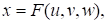
In the general case,
constructive generation can be expressed as
|
|
(3)
|
where the additional parameters
 and
 define the internal structure of the solid while preserving the
parametric order induced by the generating segment. In this case, the final
equation of the plane (triangle) will be
|

|
(4)
|
and body (tetrahedron) equation will be
|

|
(5)
|
This constructive
process does not rely on explicit surface definitions or topological
operations. Instead, the resulting solid (5) emerges as a continuous extension
of the generating entity within a higher-dimensional parameter space. Such
inheritance of parametric structure ensures consistency of internal
organization and provides a natural basis for subsequent Boolean evaluation
based on pointwise Boolean conditions.
Distinction from
unstructured point clouds
The fundamental
differences between parametric point-based solids and unstructured point clouds
are summarized in Table I.
Table 1. Semantic and structural
differences between parametric point-based solids and unstructured point clouds
|
№
|
Aspect
|
Parametric point-based solids
|
Unstructured point clouds
|
|
1
|
Geometric origin
|
Generated procedurally from a
bounded parametric domain
|
Acquired or stored as a finite set
of spatial samples
|
|
2
|
Relation to parameters
|
Explicit correspondence between
points and parameter values
|
No parametric correspondence
|
|
3
|
Generative rule
|
Defined by an analytic
point-generation mapping
|
Absent
|
|
4
|
Ordering principle
|
Induced by the structure of the
parameter space
|
Undefined; points are independent
|
|
5
|
Reproducibility
|
Geometry is reproducible through
parameter re-evaluation
|
Geometry is not reproducible without
original data
|
|
6
|
Boundary and interior
|
Unified within a single parametric
formulation
|
Not distinguished without additional
processing
|
|
7
|
Topological information
|
Not explicitly defined; replaced by
parametric order
|
Absent or reconstructed post hoc
|
|
8
|
Suitability for pointwise Boolean
evaluation
|
Naturally supports pointwise
classification and filtering
|
Requires auxiliary structures or
preprocessing
|
Unlike unstructured
point clouds commonly used in remote sensing and reconstruction tasks [2, 3],
parametric point-based solids preserve explicit correspondence between points
and parameter values. As shown in Table 1, parametric order replaces
topological adjacency as the primary organizing principle, which allows
geometric meaning to be preserved without explicit connectivity [6].
Although both
representations consist of discrete point sets, parametric point-based solids
differ fundamentally from unstructured point clouds.
Parametric point-based
representation:
• preserves explicit correspondence between points and parameters;
• allows reproducible geometry through re-evaluation;
• encodes intrinsic ordering independent of spatial proximity.
Unstructured point clouds:
• lack generative rules;
• do not preserve parametric identity;
• require additional processing to recover geometric meaning.
This distinction is
critical for subsequent Boolean operations and further processing. Parametric
order provides a stable reference frame for classification, filtering, and
interpretation of points without reconstructing adjacency relations or mesh
connectivity.
Parametric order and
the absence of topology
A key feature of the
parametric point-based representation is the absence of explicitly defined
topology. Surfaces, edges, and vertices are not treated as primary entities.
Instead, geometric features arise implicitly from the structure of the
parameter domain and the behavior of the mapping
.
The ordered nature of
the point set plays a central role in preserving geometric meaning. In this
framework, parametric order replaces topological adjacency as the primary
organizing principle. Rather than encoding connectivity explicitly, geometric
coherence is maintained through the continuity and structure of the parameter
space. This shift allows complex solids to be represented and processed without
introducing topological artifacts or degeneracies.
Computational
implications
From a computational
perspective, the parametric point-based representation is well suited for
scalable evaluation.
Since points are
generated independently, the model naturally supports parallel computation and
GPU-based evaluation. Sampling density can be adjusted adaptively by
controlling the discretization of the parameter domain without modifying the
underlying representation.
These properties are
particularly important for subsequent Boolean operations, where large numbers
of points must be classified efficiently. The absence of explicit topology and
surface reconstruction reduces numerical instability and enables robust
processing of geometrically complex solids, including objects with intricate
internal structures.
The parametric
formulation also enables controlled variation of internal point distribution
through parameter-dependent functions, allowing internal structure to be
adjusted independently of external geometry. While this capability is not
explored algorithmically in the present work, it provides a natural extension
of the proposed framework toward modeling heterogeneous solids and structured
interiors.
Unlike boundary-based
and constructive solid geometry approaches, the proposed parametric point-based
representation does not rely on explicit boundary topology or operation trees.
Boolean operations are interpreted procedurally through pointwise evaluation
rather than through topological reconstruction or tree traversal, which
distinguishes the present framework from classical solid modeling paradigms.
Within the parametric
point-based framework, Boolean operations can be interpreted as constraints
imposed on the process of point generation and evaluation rather than as
explicit geometric transformations of solid models. Since each solid is defined
by a bounded parametric domain and a corresponding point-generation mapping,
Boolean combinations naturally arise through selective inclusion or exclusion
of points based on predefined conditions.
In this interpretation,
a Boolean operation does not alter the parametric mapping itself, nor does it
require modification of the generation procedure. Instead, logical conditions
govern whether a point generated from the parameter domain is retained in the
resulting model. These conditions are not treated as independent geometric
objects, but as Boolean criteria evaluated during point generation or pointwise
classification.
Formally, let a
point-based solid be generated by a mapping
|

|
(6)
|
A Boolean result can
then be expressed as
|

|
(7)
|
where
 denotes a Boolean condition evaluated independently for each point.
The introduced
Boolean condition does not imply the existence of an explicit parametric
representation of the Boolean result and does not prescribe how the condition
 is computed. Such pointwise Boolean evaluation represents an
interpretative abstraction implementing logical filtering of points at the
evaluation stage, enabling Boolean operations without explicit intersection
computation, but at the cost of analytic closure of the resulting object.
Types of pointwise
Boolean conditions
The proposed
interpretation of Boolean evaluation (7) is deliberately
formulation-independent and accommodates a wide range of computational
realizations. In practice, Boolean conditions may be defined through different
evaluation mechanisms, including:
1. Spatial relations between solids. Boolean conditions based on
inside–outside classification with respect to other solids.
2. Analytic conditions. Logical expressions derived from analytic
descriptions of geometric primitives or parametric constraints.
3. Implicit membership functions. Evaluation of signed distance
fields or implicit functions during point classification.
4. Procedural and GPU-based evaluation. Pointwise Boolean evaluation
implemented in procedural code or shader-based pipelines.
Although these
mechanisms differ in implementation, they share a common conceptual structure:each generated point is evaluated independently with respect to Boolean
conditions, and its inclusion in the final model is determined accordingly.
Locality of Boolean
evaluation and robustness
A key characteristic
of the proposed pointwise Boolean evaluation is the absence of explicit
intersection computation between surfaces or volumetric domains. Rather than
constructing intersection curves, recomputing boundary topology, or performing
topological repair, Boolean evaluation is performed locally at the level of
individual points.
This locality has
several important consequences:
1. Numerical robustness. Degeneracies associated with surface-surface
intersections are avoided.
2. Algorithmic simplicity. Boolean evaluation reduces to pointwise
classification without global geometric reconstruction.
3. Scalability. Independent evaluation of points naturally supports
parallel computation and GPU [13] acceleration.
These properties
distinguish pointwise Boolean evaluation from boundary-based Boolean
algorithms, where global topological consistency must be maintained explicitly.
Parametric
interpretation of Boolean results
Parametrically, the
result of a Boolean operation corresponds to a constrained subset of the
original generation domain. Although this subset is generally not expressible
as a closed-form parametric mapping, the ordered structure of the point set
preserves the generative semantics of the model at the level of individual
point identities.
Each retained point
maintains its parametric identity, which enables further interpretation,
filtering, or hierarchical composition without reconstructing explicit
geometry. As a result, Boolean operations can be applied repeatedly or combined
with other procedural transformations while maintaining consistency of the
generative process.
Importantly, the
proposed pointwise Boolean evaluation does not prescribe a specific
computational workflow. Rather, it provides an interpretative framework that
explains how different Boolean evaluation techniques- including those presented
in the subsequent computational sections- can be understood within a unified
parametric perspective. This flexibility is essential for integrating analytic
descriptions, point-based sampling, and GPU-accelerated evaluation within a
single modeling paradigm.
In this
interpretation, the described pointwise Boolean conditions may be viewed as an
abstract form of masking; however, no explicit mask object or separate masking
algorithm is introduced in the computational implementation.
The parametric
point-based framework establishes a consistent interpretation of solid modeling
that connects analytic formulation with computational practice. By representing
solids as ordered point sets generated from bounded parameter domains, the
approach eliminates explicit topology while preserving parametric meaning and
geometric interpretability.
Within this context,
Boolean operations are understood as procedural constraints applied during
point generation or evaluation. Such operations are formulated as pointwise
filtering mechanisms rather than as explicit geometric transformations or topological
constructions. This interpretation explains the numerical robustness and
scalability of point-based Boolean evaluation without requiring analytic
surface intersection or boundary reconstruction.
At the same time, the
framework makes explicit a fundamental limitation common to volumetric Boolean
modeling. While parametric order and generative continuity are preserved,
Boolean results generally do not admit closed-form parametric representations.
This trade-off reflects a broader boundary of solid modeling theory when
Boolean operations are applied to three-parameter volumetric domains.
This formulation
directly supports the computational procedures described in Section V, where
pointwise Boolean evaluation is implemented and visualized.
The analytical definition of geometric solids in
point-based calculus requires the following procedural steps:
1. Develop
a geometric modeling scheme with fixed and current points. The
geometric schematic constitutes a formal diagrammatic representation of the
underlying algorithm, specifying the complete set of graphical operations
required for the rigorous definition of a geometric solid.
2. Identify
fixed reference points. Select the initial
fixed points that form the simplex of the multidimensional space. Parameterize
the modeling algorithm.
3. Determine current
points through algorithm parameterization using point-based calculus operations
based on projection invariants:
• Three-point simple
ratio on a line.
• Line intersections.
• Parallel
translation.
• Tangent
construction.
• And other
fundamental operations.
The resulting point
equation uses coordinate vectors and reduces to a system of uniform parametric
equations. This process, called coordinate-by-coordinate computation, enables
parallel processing at the mathematical level [13].
This workflow applies universally to parameterizing geometric
objects in point-based calculus - curves, surfaces, hypersurfaces, etc. The fundamental
principle states that any geometric object, regardless of complexity,
represents an ordered point set obtainable through controlled spatial movement
of a generating point.
Let us examine several implementations of this approach for
modeling geometric solids.
Let eight independent points
 through
 be defined in ℝ³ space by their coordinates (Fig. 1). Generally, any four of these
independent points are non-coplanar.
The geometric schematic shown in Fig. 1 forms a linear
construction consisting of straight lines connecting the initial fixed points
 with current points
 ,
 ,
 .
The points
and
are intermediate points that describe motion
along four edges and two faces of the solid. The result for defining the
geometric solid is the moving point
 whose trajectory fills the space bounded by
points
.
Reference [7] established that
for geometric solids, the ambient space's dimension equals the number of
independent parameters. Therefore, parametrizing a geometric solid in ℝ³
necessitates three independent parameters
 .
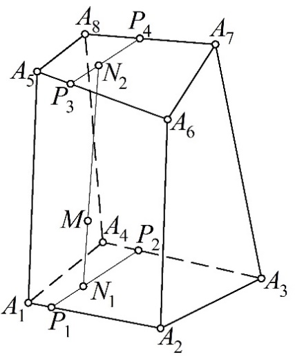
Fig. 1. Schematic diagram of a linear geometric solid determined by eight
independent points
Let
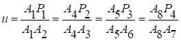 be a global
parameter defining the positions of points
 on the edges of the solid. This ensures the
coordinated traversal of each
along its designated edge.
Then the invariance of the cross-ratio of three collinear points
under parallel projection yields four pointwise equations, which constrain the
four edges of the geometric solid:
|
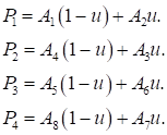
|
(8)
|
For parameter value
 ,
we obtain the initial points of the edges of the
linear geometric solid:
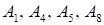 .
When
 – we obtain the terminal edge points:
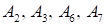 .
All intermediate parameter values
 provide the variability of current points and
consequently construct four spatial line segments representing the solid's
edges.
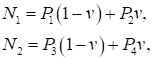
Similarly, we define current points
 using parameter
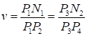 :
|
|
(9)
|
where
 by analogy with parameter
 .
After substituting point
(8) we obtain two homogeneous biparametric point sets:
|

|
(10)
|
In the general case of skew
corresponding edges, these sets define two hyperbolic paraboloids. When points
 and
 lie in two respective planes, we obtain equations
of these planes.
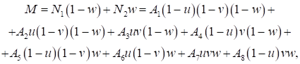
We define current point
 using parameter
 :
|
|
(11)
|
where
 by analogy with parameters
and
 .
This yields a point equation (11) of the geometric solid as a
three-parametric point set in ℝ³, uniquely
determined by the spatial configuration of eight independent initial points.
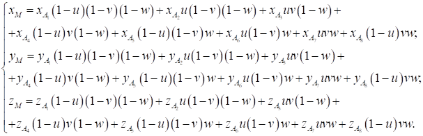
Through coordinate-by-coordinate computation, we can transform
this into a system of homogeneous parametric equations:
|
|
(12)
|
By successively fixing the limit values of parameters in equation
(11), we derive the equations of six surfaces that form the boundaries of a
linear geometric solid. This shows that the boundary representation is a
special case of our proposed point-set representation of geometric solids.
Therefore, the tools of B-rep can be directly applied to point-set
representations.
However,
this application requires a transformation of the general form into specific
boundary surfaces, which compromises the innovative potential of our approach.
Therefore, the development of geometric and computational algorithms for
implementing logical operations on solids represented by point sets is a
serious scientific challenge with obvious practical importance.
We
emphasize that this geometric scheme represents only one possible
parameterization of a linear solid, using eight independent points. Other
formulations may use four different edges or different trajectories of points,
leading to slightly different parametric equations. It is important to note
that all these formulations describe the same geometric solid. This approach to
parameterization can be easily extended to any polyhedral geometric solid.
However, as the resulting equation shows, its complexity increases with the
number of vertices. It should be noted that many geometric solids allow
parameterization not only by parameters, but also by geometric constraints.
These constraints allow calculating the coordinates of fixed and current
points.
When
applied to fixed points, geometric constraints can substantially optimize the
equation size. For current points, individual constraints or their combinations
define the solid's shape formation mechanism. We will demonstrate these
concepts through quadrilateral prism modeling.
Fundamentally, a quadrilateral prism represents a special case of
the previously defined linear geometric solid determined by eight points, where
the points become constrained through specific dependencies. We employ parallel
translation to define the current point
 (see Fig. 2).
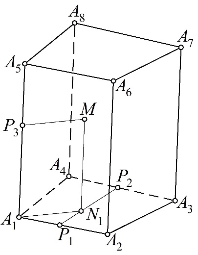
Fig. 2. Geometric Framework for Defining a Quadrilateral Prism as
a Linear Geometric Solid
In this configuration, we express the point
 in terms of parameter
 ,
yielding the following point equation:
|

|
(13)
|
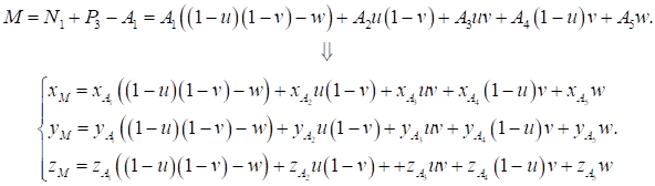
Following the established point definition methodology, we
calculate the current point
 and then perform a
parallel translation using the point formulas to complete the construction [9]:
|
|
(14)
|
This approach reduces the number of required definition points
from eight to five: four base points
( )
and one extrusion control point. The base points
can be coplanar, resulting in a prism with a flat base, or non-coplanar,
resulting in the base of a hyperbolic paraboloid. Remarkably, the fundamental
equation of the solid remains invariant - only adjustments to the input
coordinates are required.
We implement the extrusion operation through parallel translation
of current point
 using coordinate
vectors. This formulation provides a universal shape-generation tool applicable
to:
1. Extrusion of arbitrary base geometries.
2. Solutions for diverse geometric modeling problems.
3. Geometric constraints for fixed-point determination.
The vector-based parallel translation formula offers particular
advantages:
- Computational simplicity.
- Parametric flexibility.
- Unified treatment of planar/nonplanar cases.
As a demonstration, we model a quadrilateral prism with
parallelogram base, where the translation vectors directly encode the geometric
constraints of parallelism.
The most efficient implementation of our parametrization approach
utilizes three edges originating from a common vertex. We may select this
vertex from any of the prism's eight defining points. In our current
configuration (Fig. 3), we employ four non-coplanar points
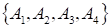 that form a three-dimensional simplex.
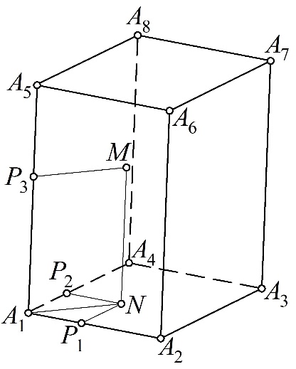
Fig. 3. Geometric framework for Defining Linear Parallelepiped
Geometric Solid
We parameterize the current points
 with three parameters
 :
|
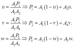
|
(15)
|
Next, we derive point
 through the point-translation formula:
|

|
(16)
|
Following the same methodology,
we obtain current point
 by applying the parallel translation formula:
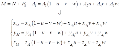
|
|
(17)
|
The derived equation defines a
three-dimensional subspace in barycentric coordinates, representing a specific
volumetric domain within ℝ³. We can
alternatively construct this geometric solid by applying the point-translation
formula to define fixed points
 ,
then substituting these into our previously established equations.
In this formula,
oblique prisms are usually represented parametrically, while rectangular prisms
are created by constraining the coordinates of four base points. The basic
equation remains the same: only the input coordinates need to be adjusted. For
example, we can model rectangular parallelepipeds by the appropriate point
configuration.
Similarly, we can
apply geometric constraints to define subsets of points of linear geometric
solid shown in Figure 1. This constraint-based approach allows us to generate
different geometric shapes from the same basic structure (Fig. 1) by changing
the geometric constraints.
The proposed modeling
approach can define not only geometric solids but also solids with cutouts,
effectively simulating the subtraction operation of Constructive Solid Geometry
(CSG). Let us consider an example of subtracting an elliptical cylinder from a
parallelepiped. Figure 4 shows the geometric scheme of this solid.
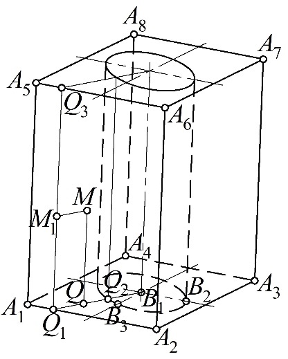
Fig. 4. Geometric scheme for parametrizing a parallelepiped with
an elliptical cutout
Based on this
geometric scheme (Fig. 4), we must define the space between the parallelepiped
and the elliptical cylinder [10]. The ellipse at the base of this cylinder has
the following point equation
|

|
(18)
|
where
 – are the points defining the major
and minor semi-axes of the ellipse, and;
 – is the angular parameter.
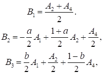
To derive the
equation of the geometric solid, it is efficient to define the points
 within the simplex
 :
|
|
(19)
|
where
 and
 – are parameters defining the major and minor
semi-axes of the ellipse, respectively.
Given the symmetry of
the modeled solid, considering one quarter of it is practical.
As an example, let us examine the
part of the geometric solid that rests on the segment
 .
In this case, the angular parameter
 belongs to the interval
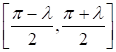 ,
where
|
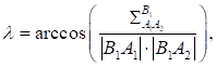
|
(20)
|
here
 – is the three-point metric operator;

 – are the lengths of segments
 and
 ,
calculated from point coordinates.
Considering (19), the
point equation of the ellipse at the cylinder base in the simplex
takes the form:
|

|
(21)
|
The current point
 lies at the intersection of lines
 and
.
Let us define a point on the line
 using parameter
 :
|

|
(22)
|
We now find the value of parameter
for which the area of triangle
 equals zero. Applying
 theorem of
point-based calculus [9] yields:
|
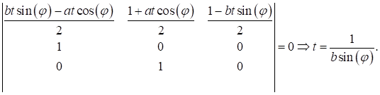
|
(23)
|
Substituting the
resulting value of parameter
into equation (23) gives:
|

|
(24)
|
We fill the internal
space of the modeled solid's base between the segment
 and the elliptical arc using parameter
 :
|

|
(25)
|
At this stage, we
have essentially obtained a two-dimensional analogue of the geometric solid—a
region bounded by three straight lines and an ellipse. Unlike traditional
methods, we define this region using a point equation rather than a system of
inequalities.
Next, we define point
 via translation:
 .
We define the current point M1 using parameter
 :
 .
We also determine the desired three-parametric current point
 through translation:
 .
After transformations, we obtain
the point equation for one of the four parts of the parallelepiped with an
elliptical cutout:
|
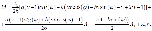
|
(26)
|
Based on the properties of
point-based calculus, equation (25) can be represented in a more compact form:
|
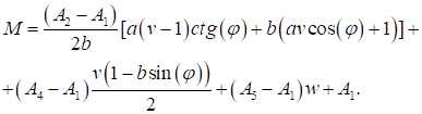
|
(27)
|
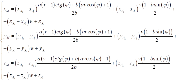
Through
coordinate-by-coordinate computation, we can transform point equation (27) into
a system of homogeneous parametric equations:
|
|
(28)
|
We visualized the
resulting model as a discrete array of 900 points to reveal the internal
structure of the space (Fig. 5). This highlights the persistent challenge
of visualizing solid geometric models, which remains an unsolved problem [11].
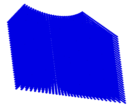
Fig. 5.
Visualization of the parallelepiped section with an elliptical cutout
Using the same
symmetry properties, we can parameterize and visualize three remaining parts of
the parallelepiped with an elliptical cutout. In the specific case where
 the method creates a circular cutout.
The disadvantage of
this method is the complexity of developing and parameterizing the geometric
scheme. However, replacing logical operations with analytical ones is a
significant advantage. This replacement opens up significant opportunities for
transferring parameterized geometric models between different CAD systems,
positioning the proposed method as a potential solution to CAD compatibility
issues.
The constructive
modeling methodology presented here has significant potential for
computer-aided design systems. Such research is already underway [14]. However,
its practical implementation currently faces limitations due to:
1. the absence of robust geometric algorithms for point-set
operations;
2. undeveloped computational methods for logical operations on
point-based representations.
Addressing these
algorithmic challenges constitutes the primary research objective of our work.
Unlike general point
cloud processing methods, the present work focuses on parametric point sets
generated analytically.
One of the most
challenging issues in geometric solid modeling with point-based calculus is the
display of models as ordered, parametrized points. This is difficult because it
is fundamentally different from what you are used to with mesh-based approaches
of faces, edges and vertices. Unlike the former, point computing characterizes
spaces in terms of their analytical rather than topological properties. This
imposes some visualization challenges on supplying designers with intuitive,
but photorealistic images of the modeled structures. These difficulties include
the lack of a mesh structure, which requires the development of specialized
algorithms for point density estimation, boundary detection, and construction
of continuous geometric representations. Furthermore, real-time visualization
management demands adaptive control of point density, surface reconstruction
and preservation of visual continuity when switching parameters. Hence
visualization of point computing demands new techniques designed with the
characteristics of point sets parametric boundaries in mind.
Prior to inventing
techniques for displaying parametric and ordered point sets in visual form, we
must consider previous scientific approaches to visualizing point cloud data
produced by remote sensing, 3D scanning, and other digital processing
techniques. Point clouds—arrayed sets of 3D points generally obtained through
lidar, stereo vision, or other 3D scanning methods—are notoriously difficult to
visualize efficiently from both a computational and algorithmic perspective.
And researchers are actively investigating these problems in computer graphics,
computational geometry, and machine learning. These state-of-the-art methods
for rendering and processing point clouds may offer a rich source of
information when designing effective visualization techniques for point computing.
Processing Noisy and
Sparse Data
Point clouds are
noisy, contain outliers and have uneven densities – it’s hard to visualize and
work with them. Data filtering and reconstruction techniques are key to solving
these problems. Among statistical methods are ray-based outlier removal (ROR)
that eliminates isolated points based on local density [15] and statistical
outlier removal (SOR) that removes points based on statistics of neighborhood
distances [16]. Deep learning also provides answers – PointCleanNet, a deep
neural network for point cloud denoising and hole filling [17], or PU-Net for
point cloud upsampling while maintaining geometric features [18].
Surface
Reconstruction
However, transforming
sparse point clouds into continuous surface meshes is still a core problem.
Reconstruction algorithms such as Poisson Surface Reconstruction – an implicit
function-based reconstruction technique [19], the Ball-Pivoting Algorithm –
which incrementally constructs meshes by rolling a ball along points [20], and deep
learning-based approaches like Pix2Vox for volumetric rendering of point clouds
[21], and Point2Mesh for neural mesh reconstruction. [22].
Rendering
Optimization
Efficient data
structures and algorithms are required by large-scale point clouds (billions of
points). Acceleration structures consist of spatial subdivision using Octrees
[23] and kd-trees [24], LOD of dynamic point cloud simplification and GPU
acceleration Splatting, rendering points as oriented quads [25], and things
like Nanite for hybrid point/mesh rendering.
Semantic Attribute
Visualization
Visualizing more
point attributes such as color, class or intensity necessitates dedicated
rendering techniques. Visualization techniques such as classification-based
false-color mapping and semantic-aware neural rendering using Neural
Point-Based Graphics [26].
Photorealistic
Rendering
State-of-the-art
photorealistic renderers adapt Phong shading to points [27] and leverage NeRF
for neural point-based view synthesis [28].
The visualization of
parametrically defined point sets in point-based calculus presents unique
challenges that traditional methods have difficulty addressing. Current
approaches often fail to address important structural design problems, such as
the implementation and visualization of set-theoretic (Boolean) operations. For
this reason, continued work in this area is both timely and essential for
pushing forward computational design.
The methods reviewed
above primarily address unstructured point clouds obtained from scanning,
sensing, or reconstruction procedures. In contrast, the point sets considered
in this work are generated analytically from parametric equations and preserve
an ordered relation to the underlying parameter domain. Therefore, several
preprocessing procedures commonly required for measured point clouds, such as
denoising, outlier removal, or surface reconstruction, are not intrinsic to the
proposed modeling framework. At the same time, rendering, shading, and
GPU-based visualization techniques developed for conventional point clouds
remain relevant at the visualization stage, since both representations
ultimately operate on discrete spatial point sets.
Imagine 3D objects as
point clouds
The simplest form of
visualization available in point-based calculus for 3D objects uses the objects
analytical description to output a sorted collection of points spaced evenly
along its parametric lines.
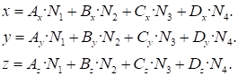
Imagine a cube
located in the first octant. These interpolation formulas for prismatic solids
calculate the point coordinates along the parametric directions u, v, and w,
each varying from 0 to 1.
|
|
(29)
|
where
 – are represent
coordinates of three distinct points defining the cube's lower base;
 – is one point in the upper base of the cube;
 ,
 ,
 ,
 – are represents a point defining the upper base
u, v, w, which vary within range 0 to 1. The type of functions is represented
by the following relationships:
|

|
(30)
|
Fig. 6
visualizes the
resulting point cloud, depicting the cube discretized into a
60×60×60 grid distributed along the parametric axes
 ,
 ,
and
 .
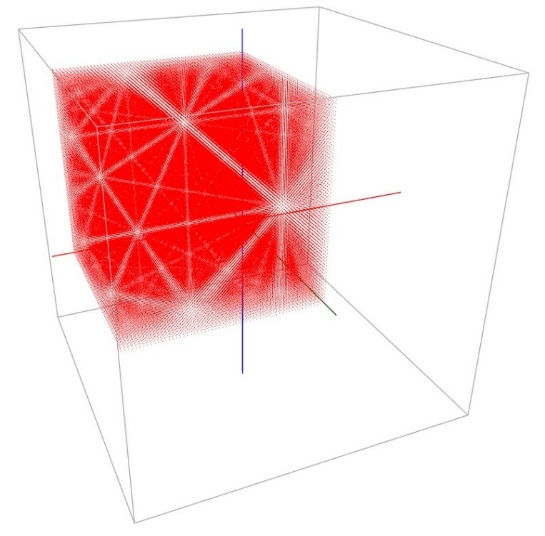
Fig. 6.
Visualization of the cube discretized into density 60×60×60
The first observation
is that the shape in question is hard to identify as a cube. Designers can see
neither its edges nor faces. Importantly, the visualization is full of
moiré patterns – artifacts of discrete 3D structures. These patterns
remain consistent after perspective shifts, lighting changes, or any other
efforts to minimize them. But clearly this visualization strategy is
insufficient.
The other option is
to ditch the organized points altogether and just generate coordinates with a
random number generator. The implementation generates the point cloud depicted
in Fig. 7 from 180,000 random points. This new visualization gets rid of
moiré.
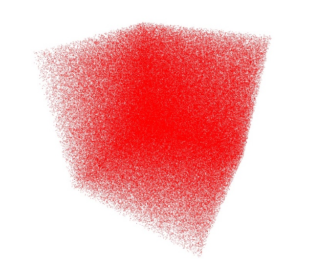
Fig. 7.
Visualization of the cube with 180000 random points
However, a
significant drawback remains: the rendering time is undesirably long and, due
to the algorithmic complexity of O(n³), strongly depends on the
number of points. As a hack, the points were randomly assigned to the cube
faces. This change enabled us to visualize a cube with 200,000 points, depicted
in Fig. 8. The complexity of this updated algorithm is O(n). This
complexity estimate characterizes the asymptotic number of pointwise operations
and should not be interpreted as a hardware-level performance benchmark.
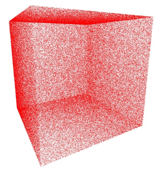
Fig. 8.
Visualization of the cube faces with 200000 random points
As shown in Fig. 8,
this visualization lets you see all faces and edges of the cube. This process
enables direct object manipulation in 3D modeling environments. The
visualization is user-controllable with two parameters: point count and point
size. In addition, the method provides object translucency with controllable
opacity, which is especially beneficial for perceiving the object’s depth
position on the screen. Fig. 9 displays a sphere drawn as a point set focused
on the surface of the sphere, created with the identical random concept.
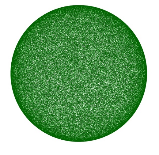
Fig. 9.
Visualization of the sphere surface with 200000 random points
The outlined approach
provides a computationally simple visualization scheme with linear asymptotic
complexity O(n)
for the considered sampling strategy. It can also be
applied to analytically defined 3D models for which point coordinates can be
generated directly from the corresponding geometric representation.
Visualization of Boolean operations on
point sets
Following the
approach described above, we explore the possibility of visualizing Boolean
operations (intersection and subtraction) between 3D objects represented as
point sets. The primary and necessary issue is locating the intersection point
subset of both interacting solids. To remedy this, let’s take a cube and a
sphere as our solids. Our solution is based on the following expressions, which
in theory should produce shape-consistent results even if the constituent
solids have different point counts.
A point
 lies inside the sphere if:
|

|
(31)
|
A point
lies inside the cube if:
|

|
(32)
|
where:
 – is the cube's center,
 – is the sphere's center,
 – is the radius.
A point meeting both
criteria, inside the cube and inside the sphere have blue color.
The second to figure
out which of these points lie on the intersection line of the surfaces of the
original solids. To fix this, we use the following approximations.
Check proximity to
the cube's faces using:
|

|
(33)
|
where
 – is a small tolerance value.
Check proximity to
the sphere's surface:
|

|
(34)
|
Points meeting both conditions
lie on the line of intersection of both surfaces and are colored yellow. Fig.
10 displays the cube (red points) and sphere (green points).
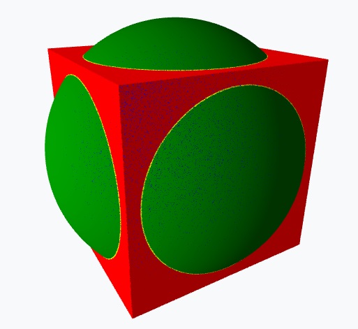
Fig. 10.
Visualization of the sphere and cube
The blue points
indicate the shared set within both volumes, while the yellow denote those
situated on the intersecting surface curve. Fig. 11-13 show visualization
results for the three Boolean operations, where we subtract the sphere from the
cube (Fig. 11), subtract the cube from the sphere (Fig. 12) and compute the
Boolean intersection (Fig. 13). For all studied Boolean operations, our
algorithm produces by clustering point subsets colored by their respective
operations. The resulting visualizations preserve a clear distinction between
the point subsets associated with the corresponding Boolean operations.
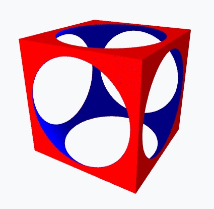
Fig. 11.
Visualization of cube sphere subtraction
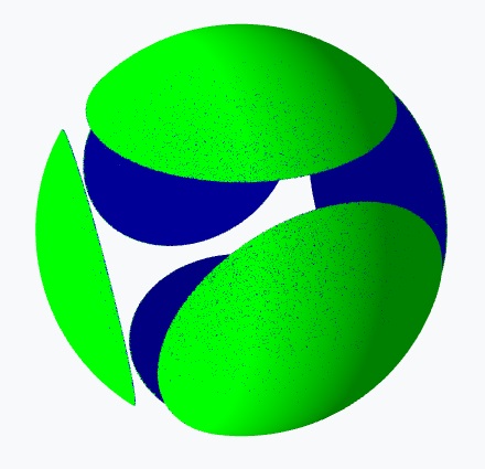
Fig. 12.
Visualization of sphere cube subtraction
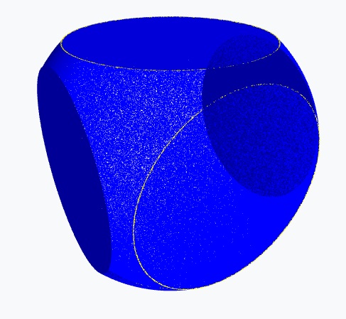
Fig. 13.
Visualization of sphere cube intersection
The current implementation is intended primarily as a
proof-of-concept demonstration of the proposed point-based Boolean workflow. A
systematic performance study, including frame-rate measurements, GPU
utilization, memory consumption, and scalability analysis for substantially
larger point sets, remains outside the scope of the present work and will be
addressed separately.
Defined by the implicit equation:

where:
– is the sphere's center,
– is the radius.
Axis-Aligned Cube:
Defined by the inequalities:
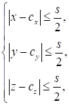
where:
– is the cube's center,
 – is the edge length.
Sphere Point Sampling:
a) Spherical Coordinates:
Points are generated using spherical parametrization:
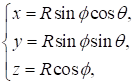
where:
 – is the azimuthal angle,
 – is the polar angle.
b) Uniform Distribution:
Random
sampling ensures uniform point density across the sphere's surface and volume.
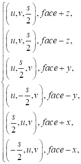
Cube Point Sampling:
a) Face-Based Sampling:
Points are generated on each of the 6 cube faces.
b) Parametric Coordinates:
For each face, two coordinates
 are randomly sampled in
 ,
and the third coordinate is fixed at
 :
Point-in-Sphere
Test:
A point
lies inside the sphere if:

Point-in-Cube Test:
A point
lies inside the cube if:

Intersection Condition:
Point satisfying both
conditions, being inside the cube and inside the sphere, are colored blue.
Surface Intersection (Boundary Detection):
•
For Sphere Points:
Check
proximity to the cube's faces using:

where
– is a small tolerance value.
•
For Cube Points:
Check proximity to
the sphere's surface:
Points satisfying both conditions lie on the intersection line of
the cube and sphere surfaces and is colored yellow.
Three Visualization Modes:
1. Intersection Mode:
• Displays points inside both the sphere and cube (colored blue).
• Highlights boundary intersections (colored yellow).
2. Cube Minus Sphere Mode:
• Displays cube points outside the sphere (red).
• Displays sphere points inside the cube (blue).
3. Sphere Minus Cube Mode:
• Displays sphere points outside the cube (green).
• Displays cube points on the surface and inside the sphere (blue).
1. Efficient Point Checks:
• Uses vectorized operations (Three.js Vector3) for fast distance calculations.
2. Buffer-Based Rendering:
• Stores point positions and colors in BufferAttribute for GPU-accelerated
updates.
3. Dynamic Updates:
• Only regenerates point clouds when parameters (e.g., cube
position, sphere radius) change.
When the cube is translated by
 :
1.
Update the cube's center:

2.
Recompute:
• Intersection tests,
• Boundary detection,
• Point cloud colors.
In brief, the algorithm:
1.
Generates point clouds for a sphere and cube.
2.
Computes intersections and surface boundaries analytically.
3.
Supports three visualization modes for Boolean operations.
4.
Supports interactive GPU-based rendering and parameter adjustment.
This algorithm is
used to visualize the models shown in Figs. 10-13.
Rendering 3D models from large point sets is a complex computer
graphics problem, particularly if we need photorealistic lighting, accurate
lighting and shadows. Unlike conventional polygonal meshes, point
representations do not have explicit connectivity or continuous surface
definition – both of which are essential for applying classical local and
global illumination models [29, 30]. In this section we describe our optical
accuracy-based approach to point cloud lighting, which tackles the problems of
surface normal estimation, illuminated region calculation and shadow
calculation.
In computer graphics,
natural rendering tries to synthesize images that look like photographs by
mimicking the physical properties of light. This technique, known as
illumination computation, calculates the interaction of light with surface
materials and yields subtle phenomena such as soft shadows, ambient occlusion,
interreflections, and specular highlights. While there are advanced pipelines
for polygonal and volumetric data, modeling models represented only as
unstructured point sets is non-trivial – particularly when points number in the
millions or billions. [29, 31]. Let us review some of the most common ways to
solve the problem of illuminating massive cloud formations.
The Surface Normal
Estimation Problem
The main challenge is simply not
having a surface. Illumination models, for example, the classic Phong and
Blinn-Phong models depend on surface normal vectors to compute the diffuse
(Lambert’s cosine law [32]) and specular components.
The local neighborhood around
each point gives the statistics to estimate these normals. Typical methods are,
for example, PCA of the k-nearest neighbors to identify the main plane and the
normal vector [33]. This estimate is very sensitive to accuracy.
•
Point Density:
Sparse regions yield unreliable normal estimates [33].
•
Noise:
Inherent noise in scanned data corrupts the calculated normal
[31].
•
Feature Preservation:
The process of estimating normal vectors can over smooth
geometry, diminishing sharp edges and fine details [33]. Inaccurate normal
vectors directly lead to erroneous lighting, manifesting as a blotchy or
"noisy" appearance rather than a smooth, continuous shading [31].
The Shadow Computation Problem
Shadows are an incredibly important realism cue, indicating
spatial relationships and location of light sources are located. Shadow
rendering is shadowing points that are blocked from a light source, usually
with ray casting (ray tracing) or comparing against depth maps (shadow
mapping).
For a point cloud, this is problematic:
•
No Explicit Occlusion Surface:
A ray cast from a point towards a light source must determine if
it intersects the "surface" of the model. However, a point cloud is a
set of discrete samples, not a continuous solid. Determining intersection
involves searching for points within a certain tolerance along the ray, which
is computationally expensive and prone to both false positives (self-shadowing
artifacts) and false negatives (light leaking through what should be occluded
areas) [31, 34].
•
Aliasing:
The discrete nature of points causes severe aliasing in shadow
boundaries, resulting in noisy, grainy shadows rather than crisp or softly
penumbral ones [34].
The Global Illumination Problem
Image naturalism requires global
illumination (GI) to mimic color bleeding (diffuse inter-reflection), and
ambient occlusion (darkening of crevices). GI algorithms (radiosity, path
tracing, photon mapping) tend to depend on surface properties and spatial
relationships that are not well-defined in a point set.
•
Lack of Connectivity:
Algorithms like radiosity require a mesh to discretize surfaces
into patches for energy transfer. Point clouds lack this connectivity, making
such methods inapplicable [29, 31].
•
View-Dependent Reconstruction:
Many point-based rendering techniques reconstruct a surface
on-the-fly from the splatting or surfeling of points. Calculating multi-bounce
light paths on a view-dependent surface is exceptionally challenging and
computationally prohibitive for large datasets [29, 31].
The scale of point sets exacerbates these theoretical problems. A
model with millions of points requires:
•
Efficient Neighbor Searches:
Normal estimation and surfel reconstruction require frequent k-NN
or radius searches, which must be accelerated by sophisticated data structures
(e.g., KD-trees, BVHs), adding pre-processing and memory overhead [33].
•
Massive Parallelization:
Achieving real-time or interactive frame rates for illuminated
point clouds almost invariably requires offloading calculations to the GPU.
Designing efficient GPU kernels for on-the-fly normal estimation and shading is
a complex task [31].
Modern approaches often represent a compromise between realism and
performance:
•
Surfel Rendering:
The algorithm represents each point as a small, oriented disc
(surfel) using a precomputed normal. Lighting is then calculated per surfel,
approximating a continuous surface. This is the technique implicitly used in
the provided code [29, 30].
•
Volumetric Approaches:
The point cloud is converted into an intermediate representation,
such as a signed distance field (SDF), which defines an implicit surface.
Well-established polygon-based lighting and shadowing techniques can then be
applied after extracting a mesh (via Marching Cubes) or directly on the volume.
•
Data-Driven and Neural Methods:
Emerging techniques use deep learning to learn a mapping from a
3D point position and its local context to a photorealistic shaded color,
potentially bypassing the explicit need for physical light simulation [30, 31,
35].
For us, the description of 3D
solids by analytical expressions – a primary strength of point modeling – make
this job much easier. We can then analytically calculate normals at each point
and store them as point attributes. This analytical information provides the
basis for the point-based lighting algorithm described in the following
section.
Core Lighting Algorithm
1. Lighting Model
Components
The algorithm implements a hybrid
lighting model combination:
Ambient Lighting:
• by Provides uniform base illumination.
• Intensity controlled parameter
 .
• Mathematical color representation:
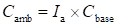 .
Diffuse Lighting (Lambertian Reflection):
• Calculated using Lambert's cosine law.
• Depends on angle between surface normal and light direction.
• Mathematical formula:

where n is the normalized surface normal vector and l is the normalized light direction vector.
2. Combined Lighting Calculation
The total illumination is computed as:

where:
• Iₘᵢₙ
is the minimum light threshold for intersection points;
• Iₐ is the ambient intensity;
• Idiff is the diffuse intensity.
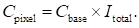
The final color is then calculated as:

3. Special Handling for Intersection Points
The algorithm implements enhanced
visibility for important regions:
Intersection Priority Lighting:
• For points identified as intersection
regions:
 (configurable).
• For regular points:
 (ambient intensity only).
• This ensures intersection areas remain
clearly visible regardless of lighting angle.
4. Normal Vector Calculation
For Sphere Points:
• Normal vector n is computed as:
 ,
where p is the point position relative to sphere center
For Cube Points:
• Normal vectors are axis-aligned based
on which face the point lies on.
• For example, points on the + X face have normal
 .
5. Light Direction
Processing
The light direction vector l is:
• Normalized to unit length:
 .
• Configurable through GUI parameters
 .
• Used uniformly across all lighting
calculations.
6. Mathematical Operations in Order
For each point in the visualization:
1.
Normal Calculation:
Compute surface normal n based on geometry.
2.
Normalization:
Ensure n is a unit
vector:
 .
3.
Dot Product:
Calculate
 (cosine of
angle between vectors).
4.
Diffuse Intensity:
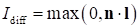 .
5.
Total Intensity:
 .
6.
Color Application:
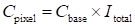 .
7. Performance Optimization
The algorithm uses:
• Buffer attributes for efficient GPU processing.
• Batch processing of lighting calculations.
• Pre-computation of normalized vectors.
• Efficient update mechanisms when
parameters change.
This lighting
approach creates a visually intuitive representation, clearly emphasizing
intersection regions while maintaining physically plausible illumination across
all surfaces. The lighting model described above is applied to the Boolean
visualizations shown in Figs. 10-13.
In addition to the presented geometric and computational
algorithms, the paper introduces a parametric interpretation of point-based
solid representation and Boolean processing. This interpretation establishes a
unified conceptual framework for understanding how ordered point sets,
generated from bounded parameter domains, support pointwise Boolean evaluation
without explicit topological construction. It clarifies the relationship
between the analytic formulation and the computational procedures demonstrated
in the paper.
The paper presents geometric and computational algorithms for
describing solids as ordered point sets with
point-based calculus and for
Boolean operations on them. Research, illustrated by examples, shows that:
1. The capability to represent solid geometric models via a single
Unified Point Equation containing information about an object’s shape,
position, and internal spatial structure.
2. The feasibility of executing Boolean operations on geometric
solids represented as ordered point sets – essential for integrating this
approach into existing geometric modeling and computer-aided design (CAD)
systems.
Key Advantages proposed algorithm:
• Mathematically rigorous intersection tests.
• Interactive rendering of the considered point-based models using Three.js.
• Interactive parameter adjustments (GUI-controlled).
• The proposed approach provides a basis for further applications in
computational geometry, collision detection, and 3D modeling.
• Future work for our solid geometric modeling approach toward
next-generation CAD systems
• Novel tools for parameterizing geometric objects, implemented
within point-based calculus.
• New methods for storing geometric information based on point
equations, capable of solving the interoperability challenge.
• Advanced algorithms for generating computational meshes for finite
element analysis.
• Vectorization of voxel models.
• Enhanced tools for performing Boolean operations on geometric
solids.
• Implementation of data-level parallelism within the mathematical
framework of point-based calculus.
• Implementation of task-level parallelism through constructive
geometric modeling algorithms based on projective and affine frameworks.
The presented computational results should be regarded as a
proof-of-concept demonstration; quantitative assessment of rendering
performance and scalability remains a subject of further study.
The study was supported by the
Russian Science Foundation, Grant No. 25-21-00003,
https://rscf.ru/project/25-21-00003/
1. MäntyläM. An Introduction to Solid Modeling, Computer Science Press, Rockville, MD,
1988
2. Kulawiak
M. Comparison of 3D Point Cloud Completion Networks for High Altitude Lidar
Scans of Buildings. Photogrammetric Engineering and Remote Sensing. 90(1)
(2024) 55-64. https://doi.org/10.14358/pers.23-00056r2
3. Un
Nabi Jafri S.R., Rehman Y., Faraz S.M., et al., Development of Georeferenced 3D
Point Cloud in GPS Denied Environments Using Backpack Laser Scanning System, Elektronika
ir Elektrotechnika. 27(6) (2021) 25-34. https://doi.org/10.5755/j02.eie.29063
4. Li
Ya., Tang K., Zeng L. A Voxel Model-Based Process-Planning Method for Five-Axis
Machining of Complicated Parts, Journal of Computing and Information Science in
Engineering. 20(4) (2020). https://doi.org/10.1115/1.4046589
5. Tian
Y., Xiao Sh., Zhang R., et al. Local dynamic update methods for 3D geological
solid structure model and voxel model, Earth Science Informatics. 17(1) (2024)
841-851. https://doi.org/10.1007/s12145-023-01183-5
6. Andújar
C., Brunet P., Chica A., et al. Solid Modelling for Manufacturing: From
Voelcker’s Boundary Evaluation to Discrete Paradigms, Computer-Aided Design.
152 (2022) 103370. https://doi.org/10.1016/j.cad.2022.103370
7. Konopatskiy
E.V., Bezditnyi A.A., Lagunova M.V., Naidysh A.V. Principles of solid modelling
in point calculus, Journal of Physics. 012063 (2021).
https://doi.org/10.1088/1742-6596/1901/1/012063
8. Mortenson
M.E. Geometric Modeling, John Wiley & Sons, New York, 1985
9. Balyuba
I.G., Naidysh A.V., Konopatskiy E.V., Rotkov S.I., Bezditnyi A.A. Theoretical
Foundations of the Point calculus as a Mathematical Apparatus for Geometric and
Computer Modeling, Vestnik komp'yuternyh i informatsionnyh tekhnologiy. 20(2)
(2023) 3-15. https://doi.org/10.14489/vkit.2023.02. pp.003-015 [in Russian]
10. Konopatskiy
E.V., Bezditnyi A.A. Solid modeling of geometric objects in point calculus,
CEUR Workshop Proceedings. 3027 (2021) 666-672.
https://doi.org/10.20948/graphicon-2021-3027-666-672
11. Konopatskiy
E.V., Bezditnyi A.A. The problem of visualizing solid models as a
three-parameter points set, Scientific Visualization. 14(2) (2022) 49-61.
https://doi.org/10.26583/sv.14.2.05
12. Konopatskiy
E.V., Bezditnyi A.A. Modeling and Visualization of Complex Shaped Surfaces
Using Interpolation Curves, Scientific Visualization. 16(4) (2024) 1-10.
https://doi.org/10.26583/sv.16.4.01.
13. Konopatskiy
E.V. Theoretical Basis of Mathematical Apparatus for Parallel Computing
Implementation in Computer-Aided Design Systems, Programming and Computer
Software. 50(5) (2024) 335-342. https://doi.org/10.1134/S0361768824700142
14. Bezditnyi
A.A. Implementation of the Set-Theoretic Subtraction Operation in Point
calculus, Scientific Visualization. 17(2) (2025) 97-109.
https://doi.org/10.26583/sv.17.2.07
15. Rusu
R.B., Blodow N., Marton Z.C., Soos A. Towards 3D Point Cloud Based Object Maps
for Household Environments, Robotics and Autonomous Systems. 56(11) (2008)
927-941. https://doi.org/10.1016/j.robot.2008.08.005
16. Rusu
R.B., Cousins S. 3D is here: Point Cloud Library (PCL), IEEE ICRA. (2011).
https://doi.org/10.1109/ICRA.2011.5980567
17. Rakotosaona
M.J., V. La Barbera, Guerrero P., Mitra N., Ovsjanikov M. PointCleanNet:Learning to Denoise and Remove Outliers from Point Clouds. (2020).
https://doi.org/10.48550/arXiv.1901.01060
18. Yu L., Li
X., Chi-Wing Fu, Cohen-Or D., Pheng-Ann Heng. PU-Net: Point Cloud Upsampling
Network, IEEE CVPR. (2018). https://doi.org/10.1109/CVPR.2018.00295
19. Kazhdan
M., Bolitho M., Hoppe H. Poisson Surface Reconstruction, The Eurographics
Association. (2006). https://doi.org//10.2312/SGP/SGP06/061-070.
20. Bernardini
F., Mittleman J., Rushmeier H., Silva C., Taubin G. The Ball-Pivoting Algorithm
for Surface Reconstruction, IEEE TVCG. (1999).
https://doi.org/10.1109/2945.817351
21. Xie H.,
Yao H., Sun X., Zhou S., Zhang S. Pix2Vox: Context-aware 3D Reconstruction from
Single and Multi-view Images, IEEE ICCV. (2019).
https://doi.org/10.1109/ICCV.2019.00278
22. Hanocka
R., Metzer G., Giryes R., Cohen-Or D. Point2Mesh: A Self-Prior for Deformable
Meshes, ACM Transactions on Graphics. (2020).
https://doi.org/10.1145/3386569.3392415
23. Meagher
D. Geometric modeling using octree encoding, Computer Graphics and Image
Processing. 19(2) (1982) 129-147. https://doi.org/10.1016/0146-664X(82)90104-6
24. Bentley
J.L. Multidimensional Binary Search Trees, CACM, 1975.
25. Zwicker
M., Pfister H., Van Baar J., Gross M. EWA Splatting, IEEE TVCG. 8(3) (2002)
223-238. https://doi.org/10.1109/TVCG.2002.1021576
26. Aliev K.,
Sevastopolsky A., Kolos M., Ulyanov D., Lempitsky V. Neural Point-Based
Graphics, Lecture Notes in Computer Science. 12367 (2020) 696-712.
https://doi.org/10.1007/978-3-030-58542-6_42
27. Botsch
M., Kobbelt L. High-Quality Point-Based Rendering on Modern GPUs, Pacific
Conference on Computer Graphics and Applications. (2003).
https://doi.org/10.1109/PCCGA.2003.1238275
28. Mildenhall
B., Srinivasan P. P., Tancik M., Barron J. T., Ramamoorthi R., Ng R. NeRF:Representing Scenes as Neural Radiance Fields for View Synthesis, Lecture Notes
in Computer Science. (2020) 12346. https://doi.org/10.1007/978-3-030-58452-8_24
29. SunCalc –
sunrise, sunset, shadow length, solar eclipse, sun position.
https://www.suncalc.org/ (accessed 01 September 2025)
30. SunEarthTools,
Calculation of sun's position in the sky for each location on the earth.
https://www.sunearthtools.com/dp/tools/pos_sun.php (accessed 01 September 2025)
31. Zivid,
Normals: What are they and how they help us pick better.
https://blog.zivid.com/normals, 2023 (accessed 01 September 2025).
32. Pedrotti
F.L., Pedrotti L.S. Introduction to Optics, Prentice Hall, 1993
33. Choi A.
Absence of Light: Mathematics Behind Shadow Art.
https://medium.com/students-work-in-mathematics/absence-of-light-mathematics-behind-shadow-art-5f3c2aff85c3,
2023 (accessed 01 September 2025)
34. Stamminger
M. Point Based Modelling and Rendering of Virtual Worlds.
https://www-sop.inria.fr/reves/Marc.Stamminger/pbr/, 2001 (accessed 01
September 2025)
35. Han J.J.,
Wu J.Y. EndoPBR: Material and Lighting Estimation for Photorealistic Surgical
Simulations via Physically-based Rendering.
https://arxiv.org/html/2502.20669v1, 2025 (accessed 01 September 2025)