This paper examines
the practical aspects of forming a Bézier surface on an arbitrary
spatial triangular or quadrilateral contour. P. BézierХs seminal work
[1] introduced the concept of geometric modeling of composite curves and
surfaces, as well as the conditions for the smooth conjugation of curve
segments and patches. In a book by French authors, Chapter 4 discusses P.
BézierХs geometric method. A translation of this book can be found in
[2]. Monographs and textbooks [3-11] explore various mathematical and geometric
aspects of CAGD.
Historically, the
Bézier method was preceded by the Coons method [12], which implies that
a patch is formed as a superposition of three ruled surfaces. This ensures the
computational simplicity of the method. In some cases, Bézier and Coons
patches are identical (see Section 8 hereof).
The monograph [13]
by English authors dealing with the practical aspects of constructing lines and
surfaces is best suited for a prior acquaintance with computational geometry
methods. The authors of [14] consider the geometric modeling of
three-dimensional objects with a focus on solid modeling. A brief overview of
methods for creating composite curves and surfaces can be found in the
reference manual [15]. Constructive algorithms for generating composite
G2-smooth cubic Bézier curves in space and on the plane are presented in
the articles [16-18].
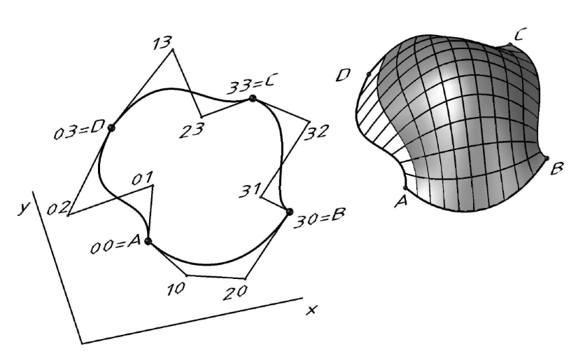
A quadrangular
patch of a cubic Bézier surface is defined by specifying sixteen
vertices 00, 01, …, 32, 33 of the characteristic polyhedron [1, 2, 3]. Each
point of the surface is associated with a radius vector
r(u, v).
For example, corner point 03 corresponds to the radius vector
r03 (Fig. 1).
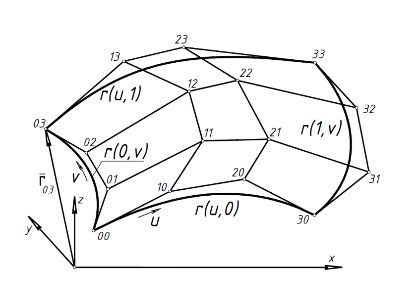
Fig. 1. Characteristic polyhedron and boundary curves of a Bézier patch
The patch equation has the form
|

|
(1)
|
where

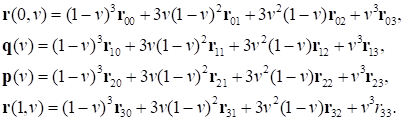
If we expand (1) and group the terms containing the v parameter, we obtain:
|
 ,
|
(2)
|
where
|
|
(3)
|
Here r(0, v) and r(1,v)
are the left and right boundaries of the patch (see Fig. 1). The curves
q (v) and p(v) that do not lie on the constructed surface are called
control curves, since they carry rows of points controlling the shape of
longitudinal generatrices (Fig. 2). Equation (2) describes the family of
longitudinal generatrices of the surface (1) for different values of the
v parameter.
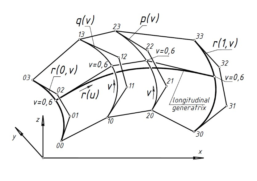
Fig. 2. Construction of a
longitudinal generatrix
The terms containing the u
parameter should be grouped to construct a family of
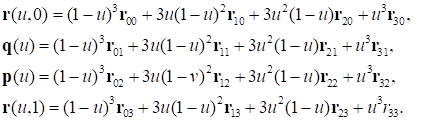
transverse generatrices in equation (1). We obtain:
|

|
(4)
|
where
|
|
(5)
|
Here, r(u,0) and
r(u,1) are the lower and upper boundaries of the patch. The
curves q(u) and p(u), which do not lie on the
surface, carry rows of points controlling the shape of the transverse
generatrices r(v) (Fig. 3). Equation (4) describes the family of
transverse generatrices of the surface (1) for different values of the
u parameter.
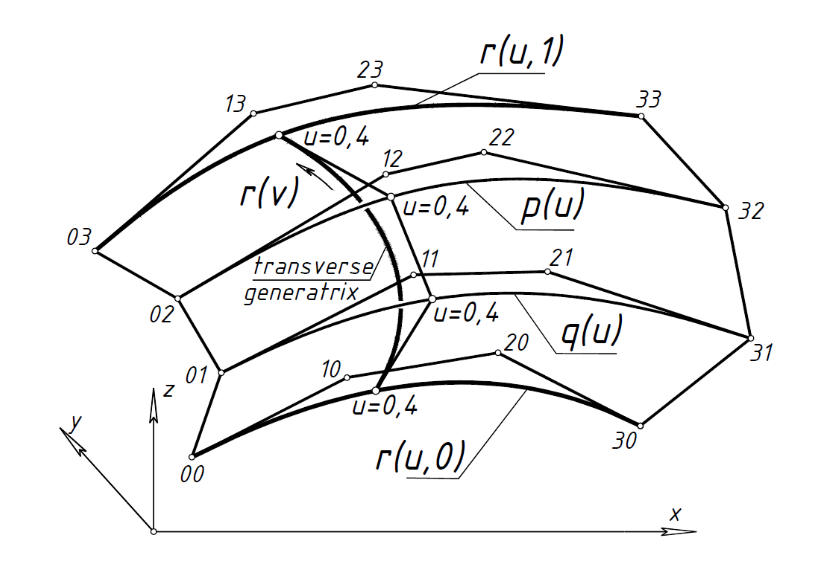
Fig. 3. Construction of a
transverse generatrix
In three-dimensional space, we define Bézier curves r(0,v),
r(1,v),
r(u,0),
r(u,1) forming a closed quadrangular contour (see Fig. 1). Our
goal is to determine the Bézier patch ФspannedХ by the given contour.
The surface is defined if there is an algorithm for constructing a set of its
longitudinal and transverse generatrices.
Generatrix
construction algorithm. We will assume that the boundary curves of the
Bézier patch and vertices 11, 12, 21, 22 of the characteristic
polyhedron are fixed (see Fig. 1).
Step 1 (construction of
longitudinal generatrices). According to (3), we construct the control curves
q(v) and p(v). Then we fix a value v=v0, for example,
v0=0.6. We mark the points r(0,v0) and
r(1,v0) on the boundary curves r(0,v),
r(1,v). We mark the points q(v0),
p(v0) on the control curves
q(v), p(v). We obtain four
points that define the characteristic broken line of the Bézier curve
r(u).
This curve is the longitudinal generatrix of the Bézier patch (see Fig.
2). We assign different values to the v parameter to generate
a family of longitudinal generatrices of the desired patch.
Step 2 (construction of
transverse generatrices). According to (5), we construct the control curves
q(u), p(u). Then we fix a value
u=u0, for example, u0=0.4. We mark the points
r(u0,0) and r(u0,1) on the boundary curves
r(u,0), r(u,1).К We mark the points
q(u0), p(u0)
on the control curves q(u), p(u). We obtain four
points defining the characteristic broken line of the Bézier curve
r(v). This curve is the transverse generatrix of the Bézier patch (see Fig. 3). We assign different values to the
u parameter to generate a family of transverse generatrices of the desired patch.
This algorithm
works for any boundary Bézier curves. These curves can be plane or
spatial; they can degenerate to a straight line or a point. For example, Fig. 4
shows a Bézier surface spanned by an arbitrarily given curvilinear
spatial contour.
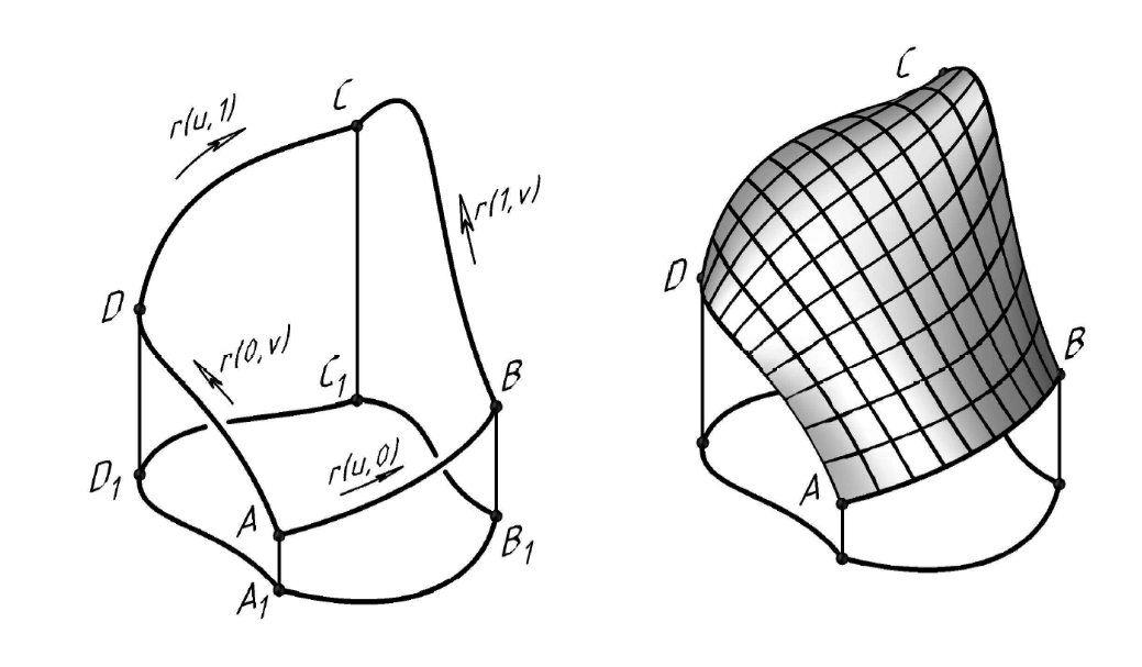
Fig. 4. Bézier surface on a
spatial contour
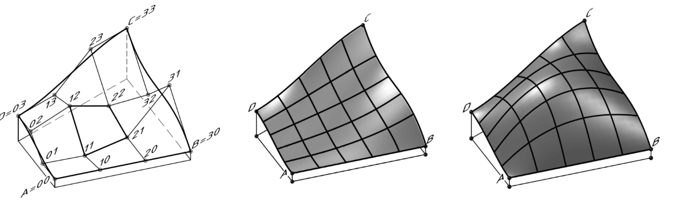
Figure 5, a shows a
characteristic polyhedron with a rectilinear boundary AB. We change the
position of control points 11, 12, 21, 22 to obtain a concave (Fig. 5, b) or
convex (Fig. 5, c) patch of the Bézier surface.
|
|
|
a)
|
b)
|
c)
|
Fig. 5. Bézier patch: a Р characteristic polyhedron; b Р concave surface; c Р convex surface
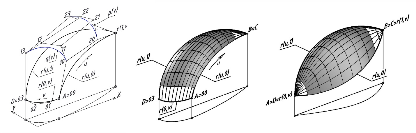
If one of the
boundaries of a quadrangular Bézier patch degenerates into a point, we
obtain a triangular patch. Let us assume for the purposes of definiteness that
the right boundary Bézier curve r(1,v) defined by
characteristic broken line 30, 31, 32, 33 has degenerated into point
B=C (Fig. 6, a). Characteristic broken lines 10-11-12-13 and 20-21-22-23 allow
drawing the Bézier control curves q(v) and p(v)
(marked in blue). We fix an arbitrary value of the v=v0
parameter. We mark the point r(0,v0) on the left
boundary curve AD. The right boundary curve has degenerated into point
B=C; therefore, r(1,v0)=B=C. We mark points
q(v0), p(v0) on the control curves. We obtain four points
r(0,v0), q(v0), p(v0),
r(1,v0)=B=C
defining the characteristic broken line of the Bézier curve r(u).
This curve is the longitudinal generatrix of the Bézier patch at
v=v0. We assign different values of the
v parameter to find a family of longitudinal generatrices of the desired patch.
Similarly, we fix different values of the u parameter to find a family of transverse generatrices.
|
|
|
a)
|
b)
|
c)
|
Fig. 6. Triangular Bézier
patches: a Р characteristic polyhedron; b Р triangular patch; c Р patch with
two degenerate boundary curves
The generatrix
construction algorithm described in Section 2 is completely preserved in the
case where two opposite boundaries of a quadrilateral contour have degenerated
into points. Figure 6, c shows a Bézier patch with degenerate boundaries
r(0,v)=A=D and r(1,v)=B=C.
If the
vertices of the characteristic polyhedron are assigned arbitrarily, the
generatrix grid of the Bézier patch is a set of spatial curves with
nonzero torsion. This solution is not technologically feasible. Let us
demonstrate the ability to generate a quadrangular patch of the Bézier
surface containing two families of plane generatrices. To this end, we impose
certain conditions on the selection of the vertices of the characteristic
polyhedron.
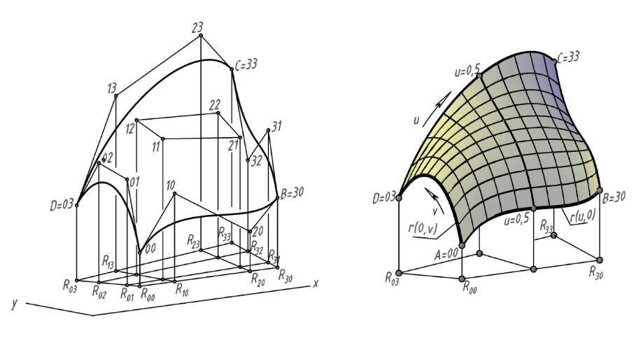
Consider the corner points A=00, B=30, C=33, D=03 for a
quadrangular Bézier patch. The orthogonal projection of the patch onto
the xy plane is an irregular quadrilateral R00R30R33R03
(Fig. 7, а).
|
|
|
a)
|
b)
|
Fig. 7. Bézier patch
with plane generatrices: a Р characteristic polyhedron with affinely
corresponding opposite sides of the plan; b Р visualization
Based on
design considerations, we define two adjacent boundaries of the patch, for
example,
r(0,v) and r(u,0). Thus, we fix eight
vertices of the characteristic polyhedron of the Bézier patch (four
corner points and two pairs of control points of the adjacent boundaries of the
patch). To define the surface, we need to define eight more vertices. If we set
these vertices randomly, we will obtain a grid of spatial generatrices with
nonzero torsion.
To obtain
the plane generatrices of the Bézier patch, we need to ensure an affine
correspondence between the opposite sides of the plan. An affine correspondence
between the left and right sides is achieved when the following ratios are
equal
|
 .
|
(6)
|
An affine
correspondence between the front and back sides of the plan is achieved when
the following ratios are equal
|
 .
|
(7)
|
Conditions
(6), (7) are satisfied with the parallel projection of one side of the plan
onto its opposite side. These conditions determine the positions of the
horizontal projections of vertices 13, 23, 31, 32 of the characteristic
polyhedron. There are no restrictions on the altitude position of these
vertices, which allows varying the shapes of the boundary curves
r(1,v) and r(u,1).
The
horizontal projections of internal control vertices 11, 12, 21, 22 are
determined at the intersection of the segments connecting the
affine-corresponding points of the opposite sides of the plan. The heights of
these vertices can be set arbitrarily.
Figure. 7,
b shows a Bézier patch generated using the specified conditions. The
plane generatrix corresponding to the value u=0.5 is highlighted in the
figure. The resulting convex-concave surface carries two families of plane
generatrices lying in vertical planes.
5. Bézier patch on a plane frame
We need to span a
Bézier surface by a plane quadrangular frame. The boundary Bézier
curves degenerate into four segments (the sides of the frame). Control points
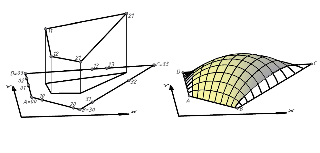
(01, 02), (10, 20), (31, 32), (13, 23) on the sides of the frame can be
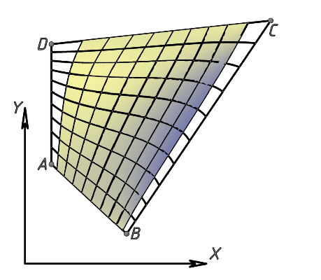
assigned arbitrarily (Fig. 8, a). The longitudinal and transverse generatrices
of the surface are determined according to the algorithm described in Section
2, resulting in a surface with non-plane generatrices (Fig. 8, b, с).
|
|
|
a)
|
b)
|
|
|
|
c)
|
Fig. 8. Bézier patch on
a plane frame: a) Р arbitrarily specified control points; b Р axonometry; с Р plan
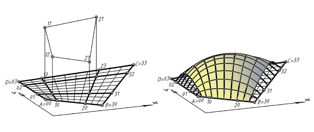
To obtain
the plane generatrices of a Bézier patch, we should ensure the affine
correspondence between the segments on the opposite sides of the frame. The control
points of adjacent sides, for example, points (01, 02) and (10, 20), can be
specified arbitrarily. Control points (31, 32) and (13, 23) are determined from
the affine correspondence between the opposite sides (Fig. 9, a). The
horizontal projections of vertices 11, 12, 21, 22 of the characteristic
polyhedron are defined at the intersection of segments connecting the
affine-corresponding points of the opposite sides of the frame. The height of
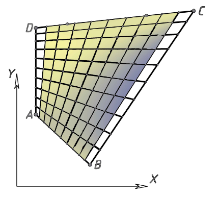
these vertices can be specified arbitrarily. We obtain a Bézier patch on
a plane quadrangular frame. This surface carries two families of plane
generatrices lying in vertical planes (Fig. 9, b, с).
|
|
|
a)
|
b)
|
|
|
|
c)
|
Fig. 9. Bézier patch
with plane generatrices: a) Р control points; b Р axonometry; с Р plan
Let the
frame be formed by plane Bézier curves, rather than rectilinear
segments. The twelve vertices of the characteristic polyhedron are fixed (Fig.
10, a). Internal control vertices 13, 23, 31, 32 can be specified arbitrarily.
Any change in the position of these vertices changes the shape of the
Bézier patch. The algorithm described in Section 2 allows constructing
an arbitrarily dense grid of longitudinal and transverse generatrices (Fig. 10,
b). Plane generatrices cannot be obtained.
|
|
|
a)
|
b)
|
Fig. 10. Bézier patch
on the plane frame of arbitrary shape: a) Р the frame is formed by
Bézier curves; b Р visualization
Let us consider the
conditions for a G1-smooth connection of two Bézier patches (Fig. 11).
According to [13, p. 195], the normal vectors to patches
ABCD=r(1)(u,v) and BMNC=
r(2)(u,v) should coincide at any point on the line of the connecting seam BC:
|
 ,
|
(8)
|
where λ is an arbitrary number. Here the superscript indicates
the patch number and the subscript indicates the variable used for
differentiation. The constant factor λ means that the
modulus of the normal vector to patches 1 and 2 may be discontinuous when
passing through the seam line.
Condition (8) is satisfied if [13, p. 197]:
|
 ,
|
(9)
|
where μ0 and μ1 are arbitrary numbers.
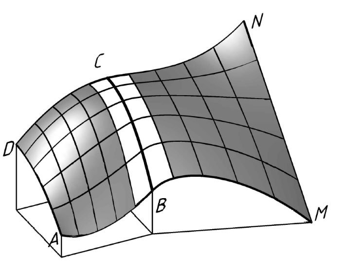
Fig. 11. Smooth connection of Bézier portions
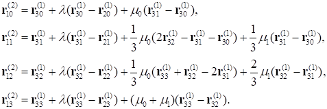
If we differentiate the equations of the patches
r(1)(u,v), r(2)(u,v)
with respect to the u and v
parameters and equate the coefficients at the same powers of
v, we obtain the well-known [13, p. 198] smoothness conditions:
|
|
(10)
|
Let us assume that
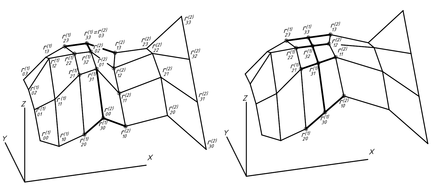
the patch r(1)(u,v) is completely defined. All
vertices r00(1) … r33(1)
of the characteristic polyhedron for this patch are fixed (Fig. 12, а). We should add the patch
r(2)(u,v) smoothly connected with the fixed patch
r(1)(u,v). The coordinates of the vertices
r10(2), r11(2),
r12(2), r13(2)
of the patch r(2) are calculated based on conditions (10). The
vertices r00(2), r01(2),
r02(2), r03(2)
defining the seam line coincide with the corresponding vertices of the patch
r(1). The remaining eight vertices of the characteristic polyhedron of the patch
r(2) can be defined arbitrarily.
|
|
|
a)
|
b)
|
Fig. 12. Characteristic
polyhedra of the Bézier ribbon: a Р smooth connection of patches
(general case); b Р smooth connection of patches (private case)
The simplest solution will be obtained if we put
μ0=μ1=0 in (10). In this case, according to (10), the edges of
the characteristic polyhedra of adjacent patches converging on the seam line
should be collinear. The ratio of the lengths of these edges should be constant
and equal to λ. The numerical
value of this parameter is assigned based on design considerations. For
example, Fig. 12, b shows the characteristic polyhedra of adjacent
Bézier patches at λ=1, μ0=μ1=0. In this case, the
longitudinal generatrices of the patches are smoothly (without a break)
connected on the seam line. This method of connecting Bézier patches can
be used if the composite boundaries between ABM and DCN are
smooth (see Fig. 11).
This method can be
used to connect Bézier patches of different shapes. For example, Fig. 13
shows a computer model of a fairing containing a triangular Bézier
patch.
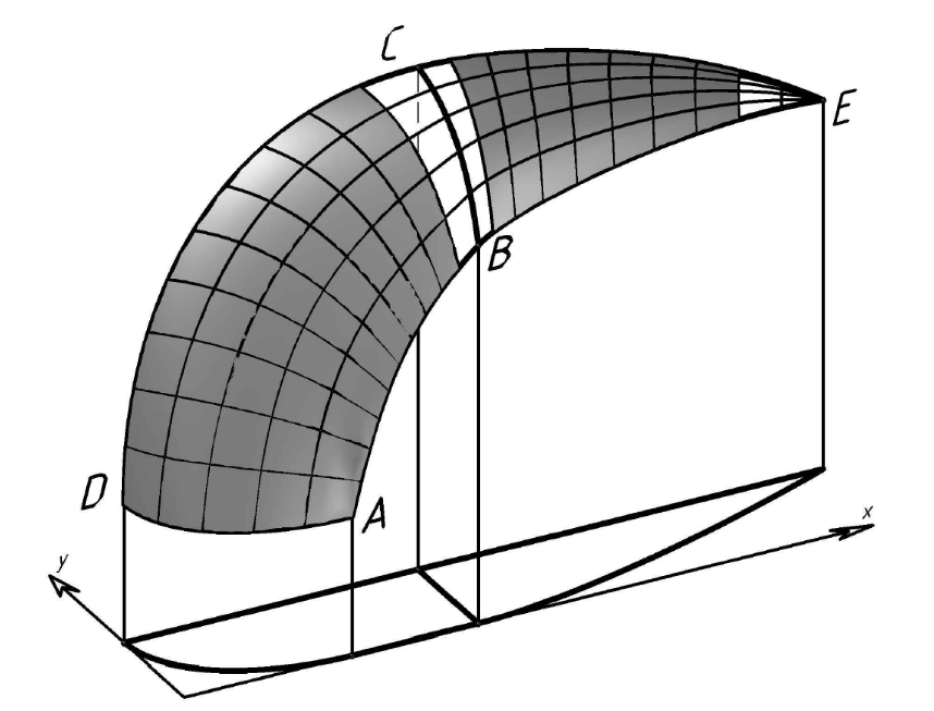
Fig. 13. Fairing
If the coefficients μ0 and μ1
are non-zero, we obtain a smooth composite surface, the longitudinal boundaries
ABM and DCN of which are broken at the connection points
B and C. In this
case, the requirement of collinearity of edges converging on the seam line is
replaced by a weaker requirement of coplanarity. According to the first
equation from (10), the edges (r20(1)Рr30(1)),
(r00(2)Рr10(2)),
(r00(2)Рr01(2))
converging at the point r30(1)=r00(2)
on the seam line should be coplanar. According to the fourth equation from
(10), the three edges converging at the point
r33(1)=r03(2)
should be also coplanar (see Fig. 12, а). The second and
third equations from (10) allow calculating the coordinates of the vertices
r11(2) and r12(2).
The fulfillment of
conditions (10) ensures the smoothness of the composite surface for any values
of the coefficients λ, μ0, μ1. In this case, the
longitudinal generatrices break on the seam line without violating the smoothness
of the surface, since at the break point on the seam line, there are three
coplanar tangents to the composite surface (the tangent to the seam line, the
tangent to the "left" longitudinal generatrix, and the tangent to the
"right" longitudinal generatrix), forming a single tangent plane. The
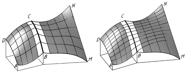
same applies to corner points B and C. For example, Fig. 14, a
shows a surface calculated for λ = 1; μ0=Р0,5; μ1=Р1.
This surface appears to have a break on the seam line BC. However, the vertical cutting planes
intersect the composite surface along smooth curves (Fig. 14, b), which
confirms that the composite surface is smooth.
|
|
|
a)
|
b)
|
Fig. 14. Smooth Bézier
ribbon with broken generatrices: a Р generatrices (Bézier curves) with a
break on the seam line; b Р section of the surface by vertical planes
Let us consider the
problem of forming a G2-smooth conjugation of two planes. G2 smoothness
(continuity) means that the curvature of the composite surface changes
smoothly, without jumps in magnitude and direction. Specifically, on the
conjugation lines of the plane and the conjugating surface, the curvature of
the latter should be zero. This requirement can be satisfied if the transition
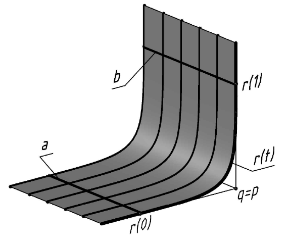
surface is defined using cubic Bézier curves. According to [4, 5], if
the control points q=p of a Bézier curve segment coincide
|

|
(11)
|
the curvature of the segment
r(t) at the end points r(0),
r (1) is equal to zero. If we shift the curve
r(t) in the transverse direction, we obtain a kinematically
defined transition surface with zero curvature on the conjugation lines
a, b with the horizontal and vertical planes (see Fig. 15,a).
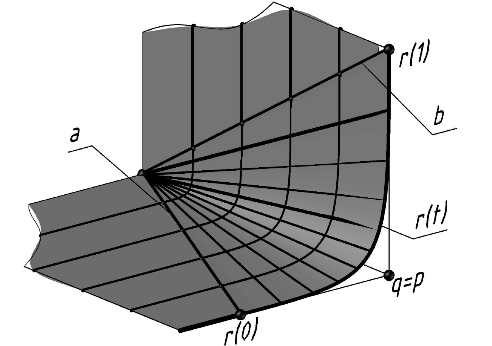
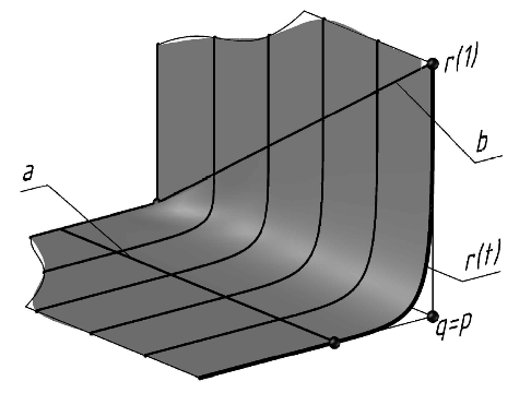
Fig. 15. Conjugation of planes
with G2 smoothness: a Р conjugation lines a, b are parallel; b Р con-jugation
lines intersect; c Р conjugation lines cross
The proposed method
of the smooth conjugation of planes can be extended to arbitrarily oriented
conjugation linesa, b. These lines intersect in Fig. 15, b and cross in
Fig. 15, c. In all cases the required G2-smooth conjugation of planes is
achieved.
According
to the Coons method [13, p. 179], the patch
r(u,v) of a surface spanned by the frame
ABCD (Fig. 16, a) is defined as a
superposition of three ruled surfaces
|
 ,
|
(12)
|
where
|

|
(13)
|
The surface r1(u,v)
passes through the "left" r(0,v) and "right" r(1,v)
boundaries of the patch. The surface r2(u,v)
passes through the "lower" r(u,0) and "upper" r(u,1) boundaries. The surface
r3(u,v) is an oblique plane based on the non-planar quadrilateral ABCD.
If we need the patch
r(u,v) to pass through the given boundaries, the
mixing functions α0, α1
should satisfy the following conditions:
|
 .
|
(14)
|
The simplest set of mixing
functions satisfying conditions (14) has the form
|

|
(15)
|
The use of linear mixing
functions (15) ensures that the Coons patches do not combine into a single
G1-smooth surface. This problem can be resolved if cubic mixing functions are
used to form the patch (12):
|

|
(16)
|
Let us
formulate the following statement (without proof): if the mixed derivatives
 at the angles of the Bézier patch
r(u,v) spanned by a quadrilateral frame ABCD
are zero ("plane angles"), the Coons patch (12), (16) spanned by the
same frame is identical to the Bézier patch. Notably, the Bézier
patch does not contain plane angles in the general case. Unlike the
Bézier patch, all angles of the Coons patch (12), (16) are plane.
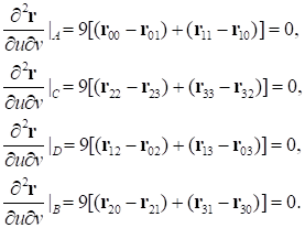
To
formulate the conditions for the existence of plane angles of a Bézier
patch, we need to find algebraic expressions for the mixed derivatives at the
angles of the patch and equate them to zero. We successively differentiate the
Bézier patch equation (2) with respect to the u and v
parameters and substitute the sets of values A{u=v=0},
B{u=1, v=0}, C{u=v=1},
D{u=0, v=1} to obtain:
|
|
(17)
|
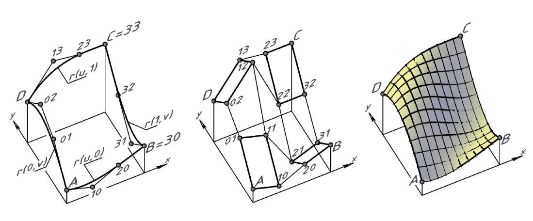
Geometrically,
conditions (17) mean that vertices 11, 12, 21, and 22 of the characteristic
polyhedron form parallelograms at the angles of the Bézier patch (Fig.
16, b). In this case, the Bézier patch acquires plane angles, and the
Bézier and Coons patches spanned by the ABCD frame coincide
identically (with an accuracy equal to the accuracy of the electronic model)
(Fig. 16, c).
|
|
|
a)
|
b)
|
c)
|
Fig. 16. Patch of a Bézier
surface with plane angles: a Р patch boundaries; b Р characteristic polyhedron;
c Р coincidence of the Coons and Bézier patches
Any software
product that supports three-dimensional graphics and allows drawing spatial
Bézier curves specified by their characteristic polyline can be used to
construct a Bézier surface. In this paper, all constructions were
performed in the AutoCAD environment using the AutoLISP programming language.
Due to the lack of licensing, the examples discussed in this paper are not
transparent. Unfortunately, the authors were unable to find a similar Russian
software product for interactive spatial construction.
According to the
proposed algorithms, a grid of longitudinal and transverse generatrices should
be drawn, followed by visualization using the "loft" command to
obtain a computer model of a surface. Each generatrix is formed as a
one-parameter set of points with any, arbitrarily small, step based on the
u or v parameter. The coordinates of the points of the generatrix are
calculated by expanding its vector equation along the x, y, z coordinate
axes. These points are connected using the "spline" command.
1. This paper
considers various options for modeling complex-shaped surfaces using cubic
Bézier curves as generatrices. The generatrix construction algorithm
described in Section 2 hereof allows defining the Bézier bicubic patch
spanned by a quadrangular or triangular closed contour generated by cubic
Bézier curves.
2. The paper
considered geometric conditions, the fulfillment of which allows obtaining a
Bézier patch with plane generatrices lying in vertical planes (see
Section 4).
3. The smoothness
conditions proposed by P. Bézier in 1972 are used to obtain a smooth
(without folds and breaks) composite Bézier surface. Under these conditions, the
generatrix grid can be broken at the seam line, while the composite surface
remains G1-smooth (see Section 6).
4. Some properties
of the Bézier curve allow forming a G2-smooth conjugation of two planes
(see Section 7).
5. It is shown that, under certain boundary conditions, the Coons and Bézier methods yield identical surfaces, which indicates a fundamental commonality between these methods (see section 8).
1. Bézier P. Numerical Control: Mathematics and Applications. John Wiley & Sons, Lon-don, 1972.
2. Bézier P. Geometric methods // Mathematics and CAD. Vol. 2. Moscow: Mir, 1989. P. 96Р257.
3. Agoston M.K. Computer Graphics and Geometric Modeling; Springer: London, UK, 2005, pp. 373-470.
4. Gallier J. Curves and Surfaces in Geometric Modeling: Theory and Algorithms; Universi-ty of Pennsylvania: Philadelphia, PA, USA, 2018, pp. 61Р114.
5. Schneider P.J., Eberly D.H. Geometric Tools for Computer Graphics; Morgan Kaufmann Publishers, Inc.: San Francisco, CA, USA, 2003, pp. 109-170, 356-358.
6. Knott G.D. Interpolating Cubic Splines; Birkhauser: Boston, MA, USA, 1999, pp. 133Р138.
7. Bartels R.H., Beatty J.C., Barsky B.A. An Introduction to Splines for Use in Computer Graphics and Geometric Modeling; Morgan Kaufmann Publishers, Inc.: Los Altos, CA, USA, 1987, pp. 6Р12, 149Р152.
8. Hoschek J., Lasser D. Fundamentals of computer aided geometric design; A K Peters / CRC Press, England, 1996, pp. 213-247.
9. Farin G. Curves and Surfaces for Computer Aided Geometric Design. A Practical Guide. Arizona State University: Academic Press, 2002, pp. 309Р364.
10. Rogers D., Adams J. Mathematical foundations of machine graphics. Moscow: Mir, 2001.
11. Pottmann H., Wallner J. Computational Line Geometry, Springer Verlag, Berlin, 2001.
12. Coons S. Ђ. Surfaces for Computer Aided Design of Space Form, MIT Project MAC, AUC-TR-41, 1967. http://publications.csail.mit.edu/lcs/pubs/pdf/MIT-LCS-TR-041.pdf
13. Fox A., Pratt M. Computational geometry. Application in design and production. Mos-cow: Mir, 1982. 304 p.
14. Golovanov N.N. Geometric Modeling. Moscow: DMK-Press, 2020. 406 p.
15. Shikin E.V., Plis A.I. Curves and Surfaces on a computer screen. Moscow: Dialog-MIFI, 1996. 240 p.
16. Korotkij V.A. Irregular curves in engineering geometry and computer graphics // Scien-tific Visualization, 2022. Vol. 14, Ь 1. P. 1Р17. DOI: 10.26583/sv.14.1.01
17. Korotkij V.A. Constructive algorithms for forming composite cubic Bézier curves in space and on the plane // Omsk Scientific Bulletin, 2022. Ь 2 (182). P. 10Р16.
18. Korotkij V.A., Studenova E.S. Construction of a spatial curve composed of rational cu-bic segments // Bulletin of the South Ural State University. Ser. Construction Engineering and Architecture. 2024. Ь 24(4). P. 72Р79. DOI: 10.14529/build240410