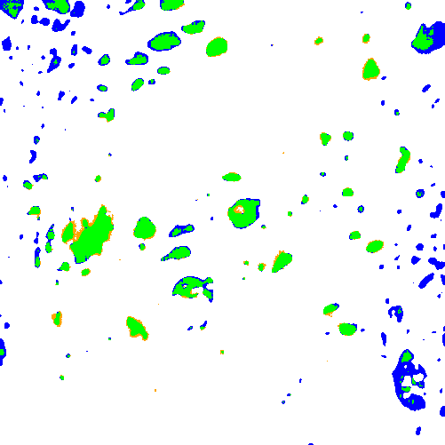
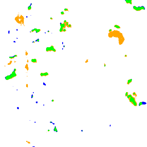
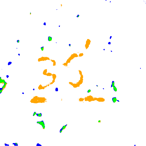
The oil and gas industry uses geological reservoir models to estimate reserves and plan production. Building geological reservoir models requires depth-based lithofacies delineation in wells, reflecting variations in sedimentation conditions and corresponding reservoir properties. In carbonate reservoirs, cavernosity is an important characteristic for lithofacies delineation. Cavernous layers contain large and spatially heterogeneous voids known as caverns. Cavernous layers require detailed analysis because they may contain significant hydrocarbon volumes; however, the feasibility of production depends on the connectivity of caverns with fractures and pores, as well as on the number, volume, and shape of the caverns [1, 2].
Various techniques support analysis of caverns. Caverns appear as low-density objects in computed tomography data of core samples [1, 3], as dark voids in optical photographs of core samples or optical borehole wall images [4], and as objects of increased electrical conductivity or acoustic scattering in borehole wall images [2, 5, 6]. These techniques differ in their analysis domains, as computed tomography reflects the internal structure of extracted core samples, photographs typically show the lateral surface of core samples from a particular viewpoint, and borehole images display measured characteristics on the borehole wall surface. In addition, the techniques differ in the ambiguities associated with interpreting objects as caverns. None of the techniques provides a precise estimate of cavernosity, and technique comparison therefore relies primarily on qualitative analysis.
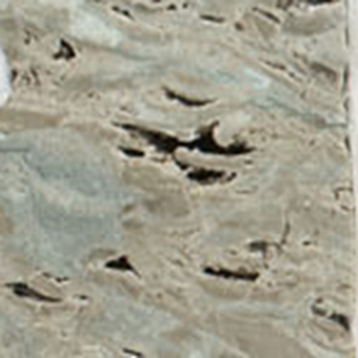
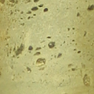
During field development, operators extract core samples from multiple wells across broad depth intervals. Core-handling procedures typically include photography, making core photographs one of the earliest and most accessible sources of information for lithofacies delineation. Photographs provide the basis for analysis of color and texture characteristics of cores [7, 8, 9, 10, 11, 12]. In particular, core photographs enable analysis of surface-visible caverns (Figure 1) and can support construction of a depth-dependent profile that qualitatively reflects variations in cavernosity. However, reliable cavern identification remains challenging, even for experts. For example, some fractures and rock chips may resemble caverns. Therefore, in the context of core photographs, it is more appropriate to refer to the detection of cavern-like objects rather than true caverns (in the geological sense) only.
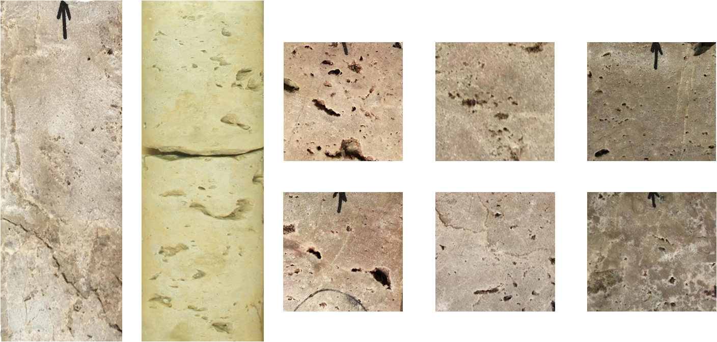
Figure 1. Cavernous core samples. The
height of the two samples on the left is 15 cm. The height of the six samples
on the right is 5 cm.
Rock
heterogeneity, non-uniform illumination during image acquisition, and the
presence of non-target dark objects increase the complexity and ambiguity of
cavern detection from photographs. This study proposes a deep-learning-based
workflow to segment cavern-like objects and construct a derived profile intended
to support lithofacies delineation. The workflow includes semi-automatic
annotation with subsequent manual refinement, model training on augmented
images for cavern segmentation, model inference on core photographs ordered by
well depth, construction and visualization of the cavernosity profile.
The
proposed workflow for cavern segmentation and cavernosity profile construction
from core photographs consists of three stages (Figure 2). The first stage
involves preparation of cavernous rock photos and cavern annotation. The second
stage splits the photographs into training and test sets, extracts patches from
core photos, and trains a deep neural network on augmented data. The third
stage extracts patches from the depth-ordered photographs, applies the
segmentation model to the extracted patches, aggregates the segmentation
results according to their positions in the original photographs, and
constructs and visualizes the cavernosity profile.
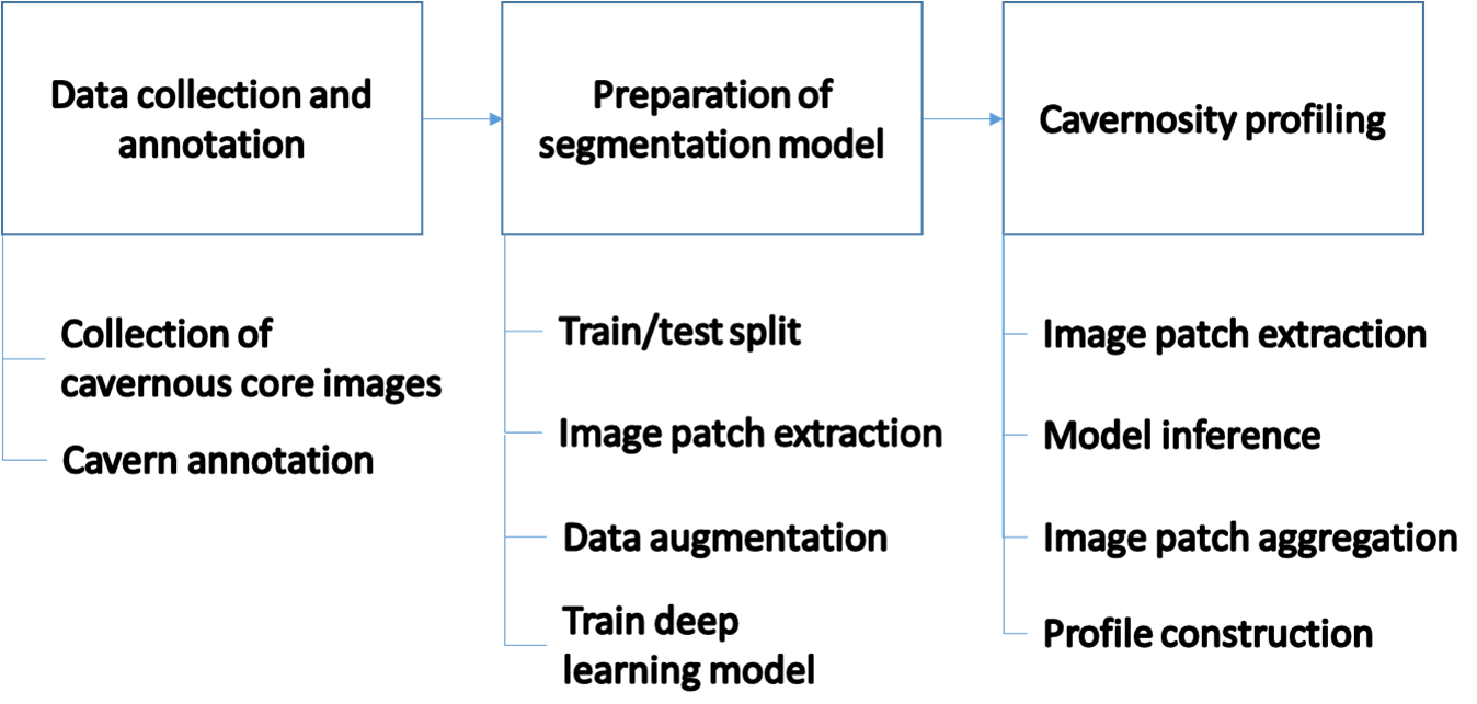
Figure 2. The workflow scheme
State and corporate standards guide the
preparation of core samples extracted from wells for storage and analysis [13,
14]. Drilling produces cylindrical core samples. In practice, operators often
slab the cores along a plane parallel to the cylinder’s vertical axis to expose
an internal cross-section unaffected by drilling. Trays then organize
cylindrical or slabbed samples according to well. Both
slabbed and cylindrical core samples are suitable for cavernosity analysis.
During
image acquisition, the setup positions core samples horizontally. The camera
mounts overhead with its optical axis perpendicular to the sample plane.
Core photographs show the lateral surface of the samples
from a single viewpoint. Core trays typically contain a depth scale bar and a
color calibration target. Although standards do not define quantitative
lighting requirements, illumination should preserve the natural color and
texture of the samples. In practice, lighting setups vary in consistency and
quality [15]. Color correction methods based on calibration targets exist [16],
but they require uniform lighting, which is not always achievable.
Cavern
annotation follows a semi-automatic workflow. Image grouping follows rock type,
imaging conditions, and the degree of rock destruction. Each image group uses
its own processing parameters. Processing includes binarization and object selection
based on shape and brightness characteristics. A geologist performed minor
annotation refinement, including removal of falsely detected objects (such as dark
mineral inclusions, fractures, and markings) and addition of missed objects.
Two additional geologists reviewed the resulting annotations to identify potential
inconsistencies.
The
binarization step applies adaptive thresholding as implemented in the OpenCV library
[17]. An adaptive threshold is determined individually for different image
regions. An adaptive threshold may be preferable to a global threshold due to varying
brightness distributions of core images. The binarization threshold is the
weighted average of the intensity values within a sliding window that moves
across the image:
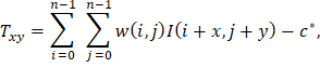
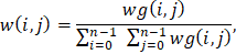
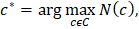
where
 is the image,
 is the window size,
 is the Gaussian-distributed weights with mean
 and variance
 ,
 is the current position of the window. The value
 corresponds to the binarization result that produces the highest number of segments
 .
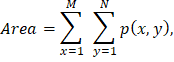
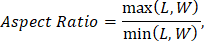
The
method selects segments from connected components based on area, aspect ratio,
and brightness. Thresholds on minimum and maximum area, maximum brightness, and
maximum aspect ratio define the selection criteria. The following formulas
calculate the area and aspect ratio of the segment:
|
|
(6)
|
|
|
(7)
|
|

|
(8)
|
|

|
(9)
|
|
|
(10)
|
|

|
(11)
|
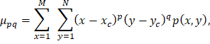
where
 ,
are the width and height of the image,
 = 1 for segment and
= 0 otherwise,
 are the length and width of the segment.
The dataset comprises 50 photographs of core samples covering 40 m
of core. The photographs represent a wide range of cavernosity appearances and
include core samples from Russian fields and the Kansas Geological Survey [18].
Splitting the data into training, validation, and test sets precedes patch
extraction. The split does not consider the data source (Russian fields or the
Kansas Geological Survey). Instead, photographs of directly adjacent depth
intervals with similar rock appearance and imaging conditions remain within the
same subset to prevent data leakage. The training, validation, and test sets
contain 36, 7, and 7 photographs, respectively. Patch extraction produces image
patches of 512 × 512 pixels, corresponding to a physical area of 5.12
× 5.12 cm2. The training set contains 1,500 patches, whereas
the validation and test sets each contain 300 patches. Patches extracted from
core photographs serve as input to the deep learning model.
The
training pipeline applies data augmentation to improve the network's
generalization capability. The augmentation includes image rotation, brightness
distribution adjustment, blurring and noise injection [19]. The augmentation
procedure randomly selects distortion parameters. To vary brightness
distribution, it applies gamma correction with a gamma value sampled from the
range [0.3, 3.0]. To simulate blur, it convolves the image with a Gaussian
kernel having a standard deviation sampled from the range [0.8, 2.6] pixels. The
procedure also adds Gaussian noise, with noise values sampled from a normal
distribution with a mean of 0 and a standard deviation of 0.15 for image
intensities normalized to the range [0, 1].
For
cavern segmentation, this study employs the U-Net architecture with a ResNet-18
backbone pre-trained on the ImageNet dataset
[20, 21]. This approach combines the robust feature extraction capabilities of
deep residual networks with the precise localization mechanism of U-Net's skip
connections. By integrating low-level details from the encoder with high-level
information in the decoder, the model effectively restores spatial
relationships.
Table 1
summarizes the model parameters. The Weighted Cross-Entropy loss function
addresses the significant class imbalance between 'cavern' and 'background'
pixels. To compensate for class imbalance, the error weight for cavern class
exceeds the error weight for the background class. The Adam optimizer updates model
weights [22]. The parameters follow the original method recommendations. The
initial learning rate is set to 0.001. The
 and
 parameters,
which control the moving averages of the gradient and its square, are set to
0.9 and 0.999, respectively. The training procedure uses a batch size of 96 and
allows up to 50 training epochs. Early stopping terminates training when the
validation loss does not improve for five consecutive epochs. During inference,
a probability threshold of 0.5 generates the binary segmentation result.
Table 1. Deep-learning model parameters
|
architecture
|
U-Net
|
|
backbone
|
Resnet-18
|
|
loss
|
Weighted
Cross-Entropy
|
|
optimizer
|
Adam
|
|
learning
rate
|
0.001
|
|
maximum
number of epochs
|
50
|
|
early
stopping patience
|
5
epochs
|
|
batch
size
|
96
|
|
binarization
threshold
|
0.5
|
For
cavern segmentation on test images, the method employs image patch extraction
with overlap. The trained model estimates the probability of each pixel
belonging to the cavern class. The aggregation step combines the probability
maps onto the image by averaging values in overlapping regions. Finally,
applying a threshold to the probability map generates the binary segmentation
result.
The
method constructs and visualizes the cavernosity profile. The profile represents
the fraction of pixels classified as cavern-like within a sliding window that
moves along depth with overlap. The sliding window size and step depend on the
analysis requirements. At the boundaries of the processing interval
(top/bottom) and in gap zones with missing images, the approach adaptively
reduces the averaging area, using up to 50% of the window size at boundary
points.
This
study assesses the segmentation model on the original and the distorted images
from the test set. The evaluation uses gamma correction
to simulate variations in brightness distribution because obtaining a
representative dataset of photographs acquired under different imaging
conditions is challenging. For the first distortion group, gamma-correction
coefficients randomly sampled from the range [1.1, 3.0] reduced overall image brightness
and decreased contrast in dark regions. For the second distortion group,
coefficients randomly sampled from the range [0.3, 0.9] increased overall image
brightness and enhanced contrast in dark regions.
The study quantified segmentation quality using the
IoU, Dice, Precision, and Recall metrics by comparing the segmentation results
with the annotations obtained using the procedure described in the “Data
Collection and Annotation” section. The IoU metric measures the ratio of the
intersection between cavern-like objects in the annotations and the
segmentation results to their union. Recall quantifies the proportion of
annotated cavern-like pixels correctly identified by the model. Precision
measures the proportion of pixels predicted as cavern-like that are also
present in the annotations. The Dice coefficient represents the harmonic mean
of Precision and Recall. Table 2 presents the metric values.
Table 2. Segmentation quality metrics for the test dataset
|
Quality metric
|
Original
|
Distortion 1
|
Distortion 2
|
|
Dice
|
0.77
|
0.78
|
0.78
|
|
IoU
|
0.62
|
0.64
|
0.64
|
|
Precision
|
0.71
|
0.72
|
0.76
|
|
Recall
|
0.84
|
0.87
|
0.80
|
The
reported metrics demonstrate that the model generalizes well to photographs
with varying brightness distributions. The Dice and IoU scores differ by no
more than 0.03 across the evaluated distortion conditions. Precision ranges
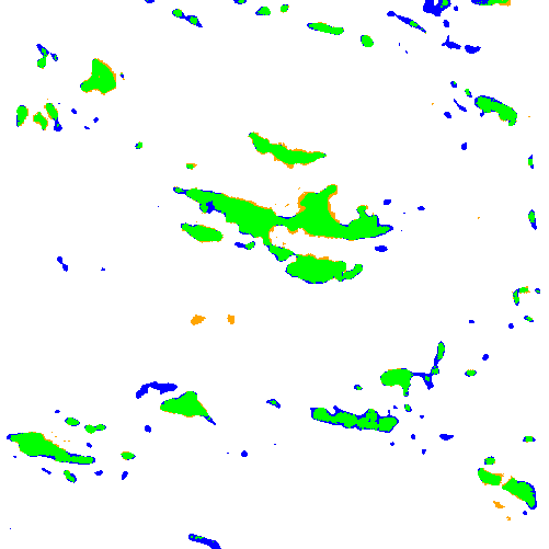
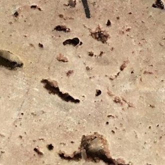
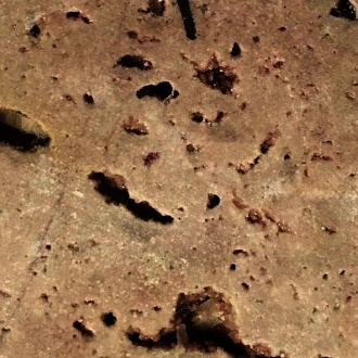
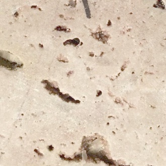
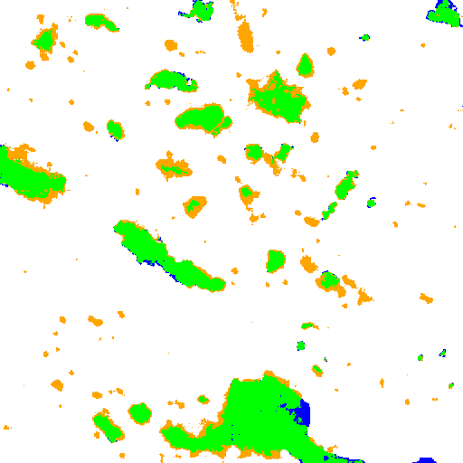
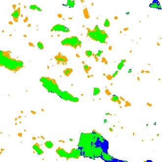
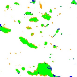
from 0.71 to 0.76, whereas Recall ranges from 0.80 to 0.87. Figure 3 shows the images
with varying brightness distributions alongside visualization maps that
highlight agreements and discrepancies between the model predictions and the
annotations. Green regions indicate the overlap between the predictions and the
annotations. Blue regions correspond to annotated areas missed by the model,
whereas orange regions indicate areas predicted by the model but absent from
the annotations.
|
Original
|
Distortion 1
|
Distortion 2
|
|
|
|
|
|
|
|
|
Figure 3. Segmentation
results for the original and gamma-corrected images
Discrepancies
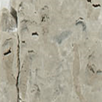
between the model predictions and the annotations primarily occur near object
boundaries and for visually ambiguous structures (Figure 4). The model
occasionally misclassifies parts of fractures or other dark objects as caverns.
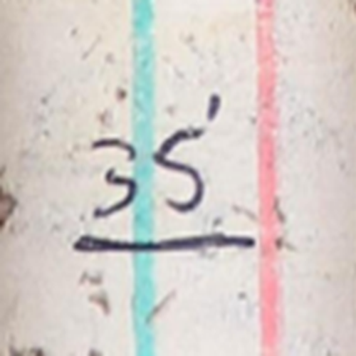
False positives also occur for dark markings present on the core samples. The
large variability in marking styles makes it difficult to represent all
possible markings in the training dataset and, consequently, to train a model
that reliably distinguishes them from large caverns. Therefore, when core
sample preparation procedures include handwritten markings, their automatic
detection and inpainting prior to cavern segmentation may improve the resulting
segmentation quality [23].
Figure 4. Examples of discrepancies between model predictions
and annotations
Figures 5 and 6 illustrate cavern segmentation results and
the derived profiles for core samples. The height of the samples is 30 cm. The
figures show both the original and distorted images. Visualization maps
displayed next to the photographs highlight agreements and discrepancies
between the model predictions and the annotations. The right side of each
figure presents cavernosity profiles constructed from the segmentation results.
The sliding window used to construct the profiles has a height of 5 mm and moves with a 1
mm step. The horizontal
scale of the profiles reflects the proportion of pixels in the sliding window
predicted as caverns. The
black profile corresponds to the original photo, the blue profile corresponds
to the first type of distortion, and the red profile corresponds to the second
type of distortion.
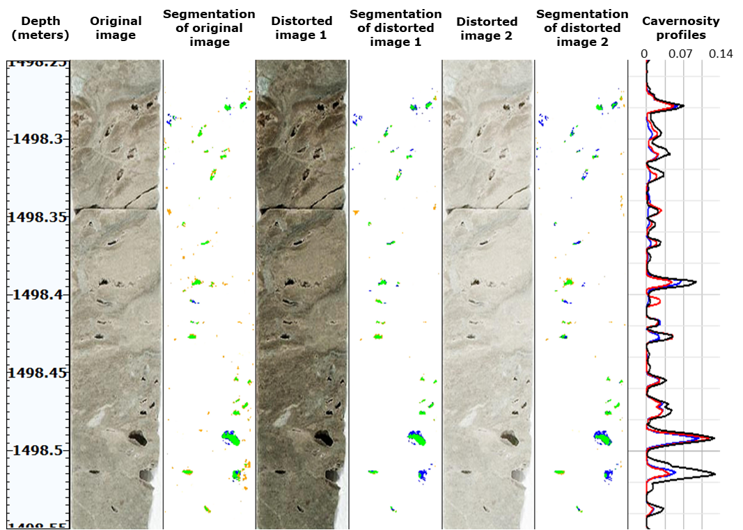
Figure 5. Segmentation results and derived profiles
for a cavernous core sample
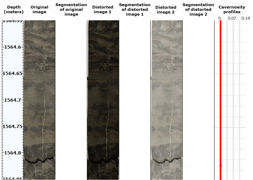
Figure 6. Segmentation results and derived profiles for a
non-cavernous core sample
Figure
5 presents profiles for a core sample exhibiting visible cavernosity, whereas Figure
6 illustrates profiles for a non-cavernous core sample. Profile values,
representing the fraction of pixels classified as cavern-like within a sliding
window, range from 0.00 to 0.14. For profiles that qualitatively characterize
cavernosity from core images, similarity across varying brightness distributions
holds greater significance than absolute values. Figures
5 and 6 show that the profiles remain similar for the original and distorted
images. Table 3 presents the pairwise Pearson correlation coefficients for the
profiles in Figure 5. For the non-cavernous sample in Figure 6, the profiles
remain close to zero. Thus, the proposed workflow enables the construction
and visualization of cavernosity profiles from core photographs with varying brightness
distributions, thereby simplifying the identification of cavernous intervals.
Geological validation of the proposed profile through
comparison with other geophysical data remains a subject for future work.
Table 3. Pairwise Pearson correlation coefficients for the profiles shown in Figure 5
|
Profile pairs
|
Original, Distortion1
|
Original, Distortion2
|
Distortion1, Distortion2
|
|
Correlation coefficient
|
0.91
|
0.91
|
0.99
|
Field
development relies on geological reservoir models that require lithofacies
description along well depth. Automating lithofacies delineation can improve the
efficiency of geologists’ work. Cavernous facies attract particular interest
because they may correspond to productive intervals. Core photographs represent
one of the most accessible sources of information for cavernosity analysis.
These photographs enable analysis of the surface manifestation of cavernosity
and support construction of a depth-dependent profile that qualitatively
characterizes cavernosity. Rock heterogeneity, varying imaging conditions,
fractures, and some artifacts complicate cavernosity analysis from photographs.
This study proposes a deep-learning-based workflow for segmentation of
cavern-like objects and construction and visualization of the cavernosity
profile. The workflow includes data collection and semi-automatic cavern
annotation, training of a deep learning model on augmented data, and
application of the model to depth-ordered photographs for cavernosity profile
construction. The method demonstrates robustness to
synthetically simulated brightness variations generated by gamma correction.
The results produced by the proposed
workflow, including the segmentation of surface-visible caverns and the
construction of a qualitative cavernosity profile, may support geologists in
lithofacies description and delineation.
1. Huang W., Cui Y., Xu F., Meng Z., Guo S., Zhang C. An innovative approach to
permeability estimation of the fractured-vuggy carbonate reservoirs based on 2D
images // Journal of Petroleum Science and Engineering, Vol. 199, 2021, 108293
(doi: 10.1016/j.petrol.2020.108293) (https://www.sciencedirect.com/science/article/pii/S0920410520313474)
2. Gavidia J. C. R., Mohammadizadeh S., Chinelatto G. F., Basso M., Ponte Souza
J. P., Portillo L. E. D., Eltom H. A., Vidal A. C., Goldstein R. H. Bridging
the gap: Integrating static and dynamic data for improved permeability modeling
and super k zone detection in vuggy reservoirs // Geoenergy Science and
Engineering, Vol. 241, 2024, 213152 (doi: 10.1016/j.geoen.2024.213152)
(https://www.sciencedirect.com/science/article/abs/pii/S2949891024005220)
3. Li B., Tan X., Wang F., Lian P., Gao W., Li Y. Fracture and vug characterization and
carbonate rock type automatic classification using X-ray CT images // Journal
of Petroleum Science and Engineering, Vol. 153, 2017, pp. 88-96 (doi:
10.1016/j.petrol.2017.03.037)
(https://www.sciencedirect.com/science/article/pii/S0920410517303911)
4. Cunningham K. J., Carlson J. I., Hurley N. F. New method for quantification
of vuggy porosity from digital optical borehole images as applied to the
karstic Pleistocene limestone of the Biscayne aquifer, southeastern Florida //
Journal of Applied Geophysics, Vol. 55, № 1-2,
2004, pp. 77-90 (doi: 10.1016/j.jappgeo.2003.06.006)
(https://www.sciencedirect.com/science/article/abs/pii/S0926985103000703)
5. Li X.-N., Shen J.-S., Yang W.-Y., Li Z.-L. Automatic fracture–vug identification
and extraction from electric imaging logging data based on path morphology //
Petroleum Science, Vol. 16, 2019, pp. 58-76 (doi:
10.1007/s12182-018-0282-6)
(https://link.springer.com/article/10.1007/s12182-018-0282-6)
6. Ausbrooks R. Quantification of vuggy porosity and lithology using borehole images, core,
and logs, Bohai Basin, Offshore China. Golden, Colorado: Master's thesis, 1999.
7. Perarnau A. Use of core photo data in petrophysical analysis // SPWLA Annual Logging
Symposium, Colorado Springs, Colorado, 2011, SPWLA-2011-Z (https://onepetro.org/SPWLAALS/proceedings-abstract/SPWLA11/All-SPWLA11/SPWLA-2011-Z/27939)
8. Khasanov I. I. Analiz tsvetnosti porod po tsifrovym izobrazheniyam kerna [Analysis of rock
color using digital core images] // Geologiya nefti i gaza, № 5, 2014, pp. 33-39
[in Russian].
9. Altunin A. E., Semukhin M. V., Mal’shakov A. V., Yadryshnikova
O. A. Sposob otsenki neftenasyshchennosti kerna gornykh porod po fotografiyam
obraztsov v dnevnom svete [A method for estimating oil saturation of rock cores
from daylight photographs of samples], 2018, RU 2654372 C1 [in Russian].
10. Abashkin V. V., Seleznev I. A., Chertova A. A., Istomin S. B., Romanov D. V.,
Samokhvalov A. F. Quantitative Analysis of Whole Core Photos for Continental
Oilfield of Western Siberia // SPE Russian Petroleum Technology Conference,
Society of Petroleum Engineers, 2020, SPE-202017-MS (doi: 10.2118/202017-MS)
(https://onepetro.org/SPERPTC/proceedings-abstract/20RPTC/4-20RPTC/450183)
11. Seleznev I. A., Abashkin V. V., Chertova A. A., Makienko D. O., Istomin
S. B., Romanov D. V., Samokhvalov A. F. Joint Usage of Whole Core Images
Obtained in Different Frequency Ranges for the Tasks of Automatic Lithotype
Description and Modeling of Rocks’ Petrophysics Properties // Geomodel,
European Association of Geoscientists & Engineers, 2020, pp. 1-5 (doi:
10.3997/2214-4609.202050090)
(https://www.earthdoc.org/content/papers/10.3997/2214-4609.202050090)
12. Seleznev I. A., Makienko D. O., Abashkin V. V., Chertova A. A.,
Samokhvalov A. F. Variograms and Co-Occurrence Matrices in Problems of
Description of Lithotypes and Modeling of Petrophysical Properties of Rocks
from Whole Core Images // Geomodel, European Association of Geoscientists &Engineers, 2021, pp. 1-5 (doi: 10.3997/2214-4609.202157117)
(https://www.earthdoc.org/content/papers/10.3997/2214-4609.202157117)
13. Porody gornye. Instruktsiya po otboru, konservatsii i khraneniyu kerna [Rocks.
Instructions for core sampling, preservation, and storage] / STO INTI 3.180.1-2025.
ANO “INTI”, 2025 [in Russian].
14. Standard Practices for Preserving and Transporting Rock Core Samples / ASTM D5079-08, ASTM
International, 2008.
15. Crawford B. Reviewing common core photography setups [Electronic resource]. Datarock, 2024.
URL: https://datarock.com.au/reviewing-common-core-photography-setups (date
accessed: 27.07.2026).
16. Potočnik M., Klemenc B., Solina F., Herlec U. Computer aided method for colour
calibration and analysis of digital rock photographs // Geologija,
Vol. 58, № 2, 2015, pp. 247-260 (doi: 10.5474/geologija.2015.020)
17. OpenCV. Image Thresholding [Electronic resource]. URL:
https://docs.opencv.org/4.x/d7/d4d/tutorial_py_thresholding.html (date
accessed: 27.07.2026).
18. Kansas Geological Survey. Kansas Core Library [Electronic resource]. University of
Kansas. URL: https://www.kgs.ku.edu/Magellan/CoreLibrary (date accessed: 27.07.2026).
19. PyTorch. Torchvision [Electronic resource]. URL: https://github.com/pytorch/vision (date
accessed: 27.07.2026).
20. Ronneberger O., Fischer P., Brox T. U-Net: Convolutional Networks for Biomedical Image
Segmentation // Medical Image Computing and Computer-Assisted Intervention –
MICCAI 2015, Lecture Notes in Computer Science, Springer, Vol. 9351, 2015,
pp. 234-241 (doi: 10.1007/978-3-319-24574-4_28)
(https://link.springer.com/chapter/10.1007/978-3-319-24574-4_28)
21. He K., Zhang X., Ren S., Sun J. Deep Residual Learning for Image Recognition //
Proceedings of the IEEE Conference on Computer Vision and Pattern Recognition
(CVPR), 2016, pp. 770-778 (doi: 10.1109/CVPR.2016.90)
22. Kingma D. P., Ba J. Adam: A Method for Stochastic Optimization // 3rd International
Conference on Learning Representations (ICLR 2015), San Diego, CA, USA, 2015
(https://arxiv.org/abs/1412.6980)
23. Dagasan
Y., Nguyen H., Grujic M. Inferring geological features masked by artefacts in
core photography using neural networks // AEGC 2021 – Australasian Exploration
Geoscience Conference, Brisbane, 2021.