Crack
detection in materials, especially in infrastructure such as roads, bridges,
and buildings, is critical for ensuring structural integrity and public
safety. Over time, various environmental factors, including weathering and load
stress, can cause cracks that, if left unchecked, may lead to structural
failure. Traditional crack detection methods rely heavily on manual inspection,
which is time-consuming, subjective, and often prone to human error.
Recent
advancements in image processing and machine learning have opened new avenues
for automating crack detection. Convolutional neural networks (CNNs), a type of
deep learning architecture, have proven particularly effective in analyzing
visual data for tasks like object recognition, segmentation, and defect
detection. By leveraging CNNs, automated crack detection systems can provide
faster, more accurate assessments of surface damage. However, these methods
often require substantial computational resources and may be difficult to
implement in real-time monitoring systems. In contrast, simpler approaches such
as binary image processing provide a cost-effective and efficient solution for
crack measurement, making them more practical for field applications.
Historically,
crack detection and measurement have relied on manual methods such as visual
inspections, calipers, or rulers. While these approaches may be
straightforward, they are labor-intensive, time-consuming, and prone to human
error. Furthermore, manual inspections are not suitable for regular, long-term
monitoring, making it difficult to track crack propagation over time. As a
result, the need for automated, precise, and efficient crack detection methods
has led to a growing interest in image processing techniques.
This
research aims to develop an image-based crack quantification that can measure
crack width and estimate crack depth. By employing noise reduction techniques
and calculating crack depth using geometric properties such as angles and
width, the system can provide a comprehensive analysis of cracks. The proposed
method offers a more objective and scalable solution than traditional
approaches, potentially improving the accuracy and efficiency of crack
detection in various applications.
1. Crack Detection Using Image Processing
Crack detection
is a critical component of structural health monitoring (SHM), and various
image-processing techniques have been proposed to automate this process. One of
the most recent approaches involves convolutional neural networks (CNNs), which
have shown considerable success in automating crack detection. Omar et al.
(2018) introduced a CNN-based method for detecting cracks in concrete
structures. Their work demonstrated that deep learning could significantly
improve detection accuracy compared to traditional edge detection and
thresholding techniques. Similarly, Zou et al. (2019) developed DeepCrack,
a CNN model designed to learn hierarchical convolutional features, resulting in
precise crack detection in various environments. These machine learning
methods, while highly accurate, require significant computational resources and
extensive training data, which may limit their practicality in real-time or
low-resource environments.
Other
researchers have explored more traditional image processing methods. Yamaguchi
and Hashimoto (2010) proposed a fast crack detection algorithm for processing
large concrete surface images using percolation-based techniques. This
grayscale-based method focuses on the rapid analysis of large-scale images,
making it well-suited for field applications where high-resolution images are
involved. However, the grayscale approach may struggle with complex surfaces or
lighting variations.
How it relates
to our work:
Our approach differs by focusing on binary image processing,
which provides a lightweight and computationally efficient alternative to
complex machine learning techniques. Instead of requiring extensive datasets
for training, we apply simple thresholding and geometric analysis, making our
method more accessible for real-time monitoring and scalable to large datasets
without significant computational overhead.
2. Crack Depth Measurement Techniques
While crack
detection has been widely studied, fewer works have focused on the accurate
measurement of crack depth. Hutchinson and Chen (2006) explored the use of
image analysis to estimate crack dimensions, including width and depth, as part
of concrete damage evaluation. Their approach combined image analysis with
manual depth measurements, highlighting the challenges of obtaining precise
depth information from 2D images.
Li et al.
(2018) took this a step further by using stereo imaging to measure crack depth
in civil engineering applications. By capturing images from slightly different
angles, they were able to create a 3D depth map, providing a more detailed
understanding of crack propagation beneath the surface. However, stereo imaging
requires specialized equipment and image processing capabilities, which may not
be feasible for many monitoring scenarios.
Another
approach is digital image correlation (DIC), which Liu and Sun (2017) applied
to quantify crack depth and width in concrete structures. DIC techniques rely
on deformation patterns to measure surface displacement and infer crack
dimensions, providing high accuracy but requiring sophisticated setups.
How it relates
to our work:
Our method offers a simpler, cost-effective alternative to
stereo imaging and DIC by estimating crack depth based on the Euclidean
distance between pixel coordinates in a binary image. Using geometric
relationships and trigonometric calculations, we derive depth information from
2D images without the need for advanced 3D reconstruction or specialized
hardware. This approach is particularly valuable for routine, large-scale
monitoring where resource efficiency is critical.
3. Euclidean Distance in Image Processing
The Euclidean
distance formula is a fundamental tool in image processing, frequently used for
measuring distances between features in an image. Duda and Hart (1972)
introduced the use of geometric relationships such as Euclidean distance in
early edge detection algorithms. This foundational concept has since been
applied in a variety of contexts, including crack measurement. Wang et al.
(2019) used the Euclidean distance between the edges of detected cracks to
calculate crack width in concrete surfaces. Their approach combines adaptive
Gaussian fitting with distance measurement, producing highly accurate width
estimates in real-world scenarios.
How it relates
to our work:
In our research, we build on the traditional use of
Euclidean distance by applying it specifically to measure crack width in binary
images. By calculating the distance between the first and last detected white
pixels in each row, we determine the crack’s width. This simple, direct
approach is well-suited for our goal of calculating both width and depth using
lightweight image processing techniques.
4. Thresholding and Binary Image Analysis
Thresholding is
one of the most widely used techniques in image processing for converting
grayscale images to binary images, where objects of interest can be isolated.
Otsu (1979) proposed a method for selecting an optimal threshold based on
gray-level histograms, which has since become a standard in image segmentation
tasks. Sahoo et al. (1988) provided a comprehensive review of various
thresholding methods, including global, local, and adaptive techniques, that
apply to a wide range of image analysis tasks.
Binary image
processing, as a result of thresholding, is often the first step in object
detection, edge detection, and feature extraction in images. It allows for the
simplification of complex images by reducing them to two colors—typically black
and white—representing the background and the object of interest, respectively.
How it relates
to our work:
We employ binary thresholding to isolate cracks from the
rest of the image, converting the input RGB image into a format that simplifies
the analysis. This method allows us to detect white pixels representing cracks,
providing the foundation for subsequent width and depth calculations. While our
method builds on traditional binary segmentation techniques, it extends these
methods by using geometric functions to estimate crack depth, which is a novel
contribution.
5. Applications in Structural Health
Monitoring
Structural
health monitoring (SHM) has increasingly relied on image-based techniques for
assessing infrastructure integrity. Choi and Shah (1997) discussed how image
analysis can be used to measure deformations in concrete specimens,
highlighting its applicability in crack growth monitoring. More recently, Zhang
et al. (2020) proposed a vision-based approach for automatic crack detection
and quantification, contributing to the development of non-destructive testing
(NDT) methods for civil engineering.
Image-based SHM
methods offer the advantage of being non-invasive, allowing for the continuous
monitoring of critical structures such as bridges, tunnels, and buildings
without the need for direct physical access. This has significant implications
for safety and maintenance, as early detection of cracks can prevent catastrophic
failure and extend the life of critical infrastructure.
How it relates
to our work:
Our research contributes to the growing field of image-based
SHM by offering a method for detecting and quantifying cracks without the need
for expensive or complex equipment. The ability to measure crack width and
depth using simple image processing techniques makes our approach a viable tool
for real-time infrastructure monitoring, especially in scenarios where cost and
computational resources are limited.
Several
studies have explored fracture detection approaches and algorithms, but few
have focused on crack width assessment, which is crucial for safety diagnosis.
We
describe a crack detection technique that improves in detecting crack width and
depth, an important aspect of safety inspection. The suggested technique
involves steps: converting the image into a binary
image, thresholding, detecting cracks, detecting distance (width) using the Euclidean
distance formula, and finally depth calculation using a simple
trigonometric formula. Its key
advantage is more precise fracture pixel extraction. This method helps analyze
the depth of cracks in an image by identifying colored pixels, calculating the
distance between them, and converting this distance into a real-world depth
measurement.
In
computer vision, effective image processing techniques are essential for
extracting meaningful information from visual data. Figure 1 shows a flow
diagram of a systematic approach to processing an input image, leveraging
Python libraries such as OpenCV and pandas.
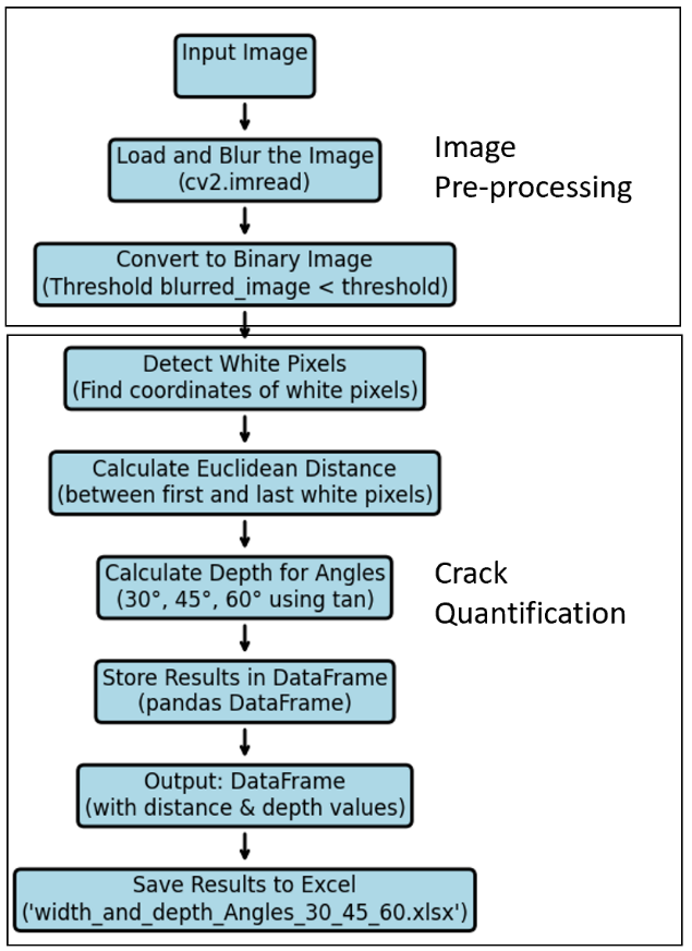
Figure 1. Flow Diagram
In the
first step, in the preprocessing phase, Gaussian blur was applied to the
original image to reduce noise and enhance the clarity of the features relevant
to crack detection. The Gaussian blur operates by convolving the image with a
Gaussian kernel, effectively smoothing the image and diminishing high-frequency
noise that could interfere with accurate analysis. This step is crucial, as it
ensures that the subsequent binary thresholding operation is performed on a
cleaner image, thereby improving the reliability of the crack detection
process.
The second
step, in the crack quantification process, involves converting a blurred image
of a cracked surface into a binary (black-and-white) image. This transformation
simplifies the analysis by reducing the complexity of the data, allowing the
cracks to be easily distinguished from the background.
The
conversion is achieved through thresholding, where a threshold level is
applied to the blurred channels of the image. In this work, a threshold level
of 4 is set, meaning that any pixel with blurred image values less than 4 is
classified as a white pixel (representing the crack), while all other pixels
are classified as black (representing the background). This process is
performed using the following condition for each pixel:
|

|
(1)
|
The
output is a binary image with white pixels representing cracks (value 255) and
a black background (value 0). This step isolates the crack features from
the surrounding material, enabling subsequent measurements of crack width and
depth.
A. Crack
Quantification Methodology
Crack
quantification is essential in various fields, such as structural health
monitoring, material science, and civil engineering, where precise measurements
of crack dimensions are crucial for assessing damage, understanding material
behavior, and predicting failure. This research employs an image-based method
to measure crack width and depth from digital images using image processing
techniques.
In this
research, crack quantification is performed using image processing techniques
to measure both the width and the depth of cracks in a given image. The
approach involves transforming an RGB image of a cracked surface into a binary
image and applying spatial measurements to quantify the crack's geometric
characteristics. Below is a detailed description of the approach used for crack
quantification.
Figure 2
shows the actual image converted into a blur image for noise reduction. We
used Gaussian Blur for noise reduction, and adjusted kernel size as we needed.
Image is
captured by camera resolution 1800 * 4000 pixels (Width * height) with 72 DPI
for both horizontal and vertical resolution.
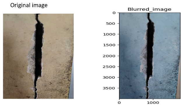
Figure 2
Actual image vs blurred image
B. Methodology for Width Calculation
Crack
width is defined as the linear measurement of the gap or fissure at its widest
point. It is a crucial parameter in evaluating the severity of cracks, as wider
cracks often indicate more significant structural distress.
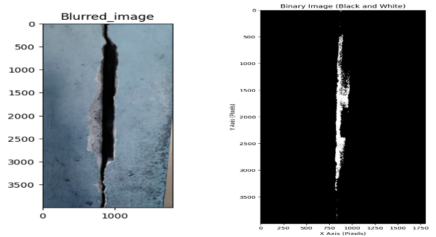
Figure 3
binary image for width calculation
Figure 3
shows the blurred image converted into a binary image for width
calculation. We analyze the binary image row by row to quantify the crack width.
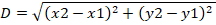
For each row, the algorithm identifies the positions of the first and last
white pixels, which correspond to the edges of the crack. The Euclidean
distance between these points is calculated to determine the crack width by
using the below formula: -
|
|
(2)
|
where
(x1,y1) and (x2,y2) are the coordinates of the first and last white pixels,
respectively. In a horizontal row, this simplifies to:
|

|
(3)
|
The
scaler factor depends on the dot per inch (DPI) or pixel per inch (PPI). Higher
PPI and DPI indicate higher clarity and quality of the image. In this
research, we used DIP resolution for images. The pixel-to-mm conversion is
mostly used for real-world data, the formula for pixel-to-mm is as follows:
|

|
(4)
|
The
calculated distance in pixels is converted to millimeters using the same scale
factor S:
|

|
(5)
|
Dmm:
distance in mm
Dpixel: distance in pixel
|

|
(6)
|
For this
paper scale factor is equal to 0.3527mm. The final formula conversion of pixel
to mm for this paper is:
|

|
(7)
|
As shown
in Figure 7, manual ruler measurements were used to validate the
pixel-to-millimeter conversion factor. The observed difference between physical
and automated measurements was typically within ±0.1 mm, which we take as the
first-order approximation of the conversion error.
Threshold and Scale Factor Selection
•
Threshold
Selection:
In the initial demonstration, a fixed threshold value of 4 was used for
binarization to illustrate the crack extraction process on a specific image.
However, for subsequent experiments and validation, Otsu’s automatic
thresholding method was employed. This approach determines the optimal
threshold dynamically from the grayscale histogram of each image, ensuring
robust separation of cracks from the background under different lighting and
surface conditions. The use of an adaptive threshold improves reproducibility
when applying the method to other datasets and shooting environments.
•
Scale Factor Calibration:
The scale factor of 0.3527 mm/pixel in this study was determined by relating
the physical size of the specimen surface (10 cm × 20 cm) to the captured
image resolution (1800 × 4000 pixels). This calibration allows
pixel-based distances to be expressed in millimeters. For other imaging setups,
the scale factor may vary depending on camera resolution, field of view, and
the distance between the camera and specimen. To ensure reproducibility across
different conditions, the scale factor can be recalibrated by including a reference
object of known dimensions within the captured image.
C. Methodology
for Depth Calculation
Crack
depth refers to the measurement from the surface of a material down to the
deepest point of the crack. Understanding crack depth is vital for evaluating
the potential for further structural failure. Crack width was
calculated based on the Euclidean distance between each row's first and last
white pixels, factoring in the angle of interest. Depth Calculation at
Specified Angles: The depth of the crack at specific angles (30°, 45°, and 60°)
is computed using trigonometric relationships. The depth d at angle θ can
be expressed as:
|

|
(8)
|
The above
formula is the original trigonometry formula for depth detection used. We
modify this as follows:-
|

|
(9)
|
• Depth at 30°:
|

|
(10)
|
• Depth at 45°:
|

|
(11)
|
• Depth at 60°:
|

|
(12)
|
Depth-to-Width Ratio Table
The
depth-to-width ratio at various angles provides a comparative view of how the
depth changes relative to the crack width. This data is useful for
understanding how angle variations affect the depth estimate for a given width.
Table 1 demonstrates that:
• At 30°, the depth is approximately 57.7% of the width.
• At 45°, the depth value is half of the width.
• At 60°, the depth is significantly greater, at 173.2% of the width.
Table 1 Ratio table
|
Angle (θ)
|
Depth-to-Width Ratio
|
Example (10 mm width)
|
Estimated Error*
|
|
30°
|
0.577
|
2.88 mm
|
±0.55 mm (≈19%)
|
|
45°
|
1
|
5.00 mm
|
±0.90 mm (≈18%)
|
|
60°
|
1.732
|
8.66 mm
|
±1.70 mm (≈20%)
|
D. Visual representation of crack quantification technique
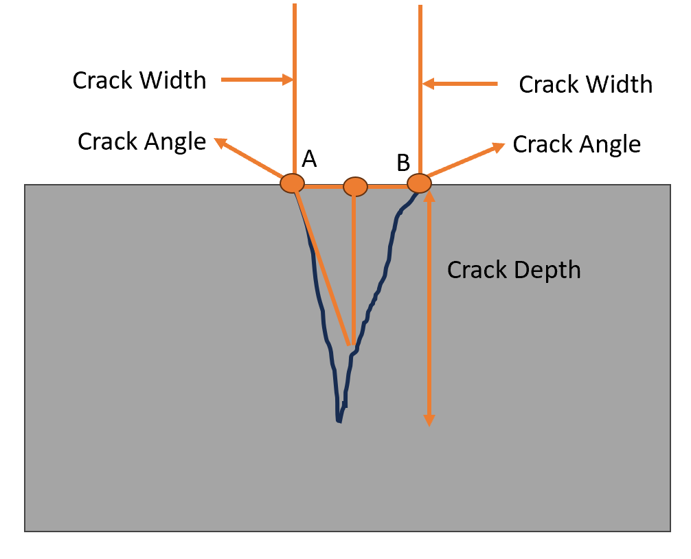
Figure 4. Visual representation of crack
Figure 4, illustrates the geometric relationships between
crack width, crack depth, and crack angle in a structural material,
such as concrete.
The horizontal distance between points A and B at the surface of the
material. The Crack Width is the horizontal distance between points A
and B, and the Crack Angle is the angle formed by the surface and the
sides of the crack at those points. It represents how much the material has
separated horizontally due to the crack. This is one of the critical parameters
in crack analysis because it helps to quantify the extent of damage at the
surface level. In real-world analysis, this crack width is measured in
millimeters (mm) using techniques such as image analysis or direct measurement.
The vertical distance from the material's surface down to the crack's
deepest point. This parameter is essential because it determines how deep the
crack has penetrated the material, which directly affects the component's structural
integrity. Deeper cracks pose a greater risk to the stability of the structure.
Crack depth is usually estimated using trigonometric relationships between the
width and the angle of the crack, or by non-destructive testing techniques such
as ultrasonic testing or radiography. The angle formed between the surface of
the material and the sides of the crack, at points A and B. The
crack angle helps to estimate the depth of the crack using trigonometry.
For example, the steeper the crack angle (closer to 90°), the deeper the crack
for a given width. Typical crack analysis involves assuming a fixed crack angle
(such as 45°) or measuring it through detailed inspection or modeling.
Points A and B
are at
the edges of the crack where the separation begins at the surface. From these
points, the crack extends downward into the material, forming a triangular
shape. By measuring the crack width and knowing the crack angle,
the depth of the crack can be calculated using trigonometric relationships. For
example, assuming a 30° angle, the depth (h) can be approximated by using the
formula:
|
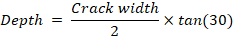
|
(13)
|
The wider
the crack and the steeper the angle, the deeper the crack will extend into the
material. Crack Width and Crack Depth are crucial indicators for
assessing the severity of cracks in structures. Wider and deeper cracks may
indicate more severe damage, requiring immediate attention. Crack Angle
affects the way forces are distributed across the crack and determines the
depth of the crack to its width.
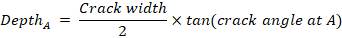
This formula 13 assumes symmetrical angles (the same on both
sides) and horizontal distance to the adjacent side in a right triangle
(known as tangent function). If the angles are different at A and B,
then you would need to calculate the depth for each side separately and add
them:
For side A:
For side B:
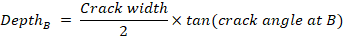
Finally,
sum the depths from both sides of the crack angles at A and B are different:

This section
presents the experimental results of the crack width and depth measurements
obtained through image processing techniques, including binary thresholding and
Euclidean distance calculations. The results are displayed in both tabular and
graphical formats, followed by a discussion that interprets the findings,
highlights their significance, and compares them with previous research.
Table 2 Result
|
Row
|
Euclidean Distance (mm)
|
Depth @ 30° (mm)
|
Depth @ 45° (mm)
|
Depth @ 60° (mm)
|
|
0
|
9.525
|
2.749631
|
4.7625
|
8.248892
|
|
1
|
9.525
|
2.749631
|
4.7625
|
8.248892
|
|
2
|
10.23056
|
2.953307
|
5.115278
|
8.859921
|
|
3
|
5.997222
|
1.731249
|
2.998611
|
5.193747
|
|
4
|
6.35
|
1.833087
|
3.175
|
5.499261
|
|
5
|
6.35
|
1.833087
|
3.175
|
5.499261
|
|
6
|
5.644444
|
1.629411
|
2.822222
|
4.888232
|
|
7
|
4.938889
|
1.425734
|
2.469444
|
4.277203
|
|
8
|
4.233333
|
1.222058
|
2.116667
|
3.666174
|
|
9
|
6.35
|
1.833087
|
3.175
|
5.499261
|
A. Crack Width and Depth Measurements
Table 2 and
Figure 5 provide the measured crack width and corresponding depth estimates
for cracks detected in a concrete structure. The values are
extracted from an image analysis, where each row in the table represents the
measurement data for cracks detected in consecutive rows of the image. The data
set comprises 10 samples, each showing how the calculated crack depth varies as
a function of the crack angle and the Euclidean distance.
The
results highlight the variability of crack width and depth across different
rows and demonstrate the impact of measurement angles on crack depth estimation.
The
Euclidean Distance for each sample, the Euclidean distance remains relatively
consistent with some variation across the samples. It ranges between
approximately 5 mm and 15 mm.
Depth @ 30°,
This column represents the estimated crack depth
when viewed at an angle of 30 degrees. Depth is derived from the width using
trigonometric principles. For instance, in row 0, the estimated depth at 30° is
2.749631 mm. In row 3, the depth is 1.731249 mm.
Depth @ 45°,
This column lists the estimated depth of the crack
when viewed at a 45-degree angle. The depth increases compared to the 30°
estimate, reflecting the trigonometric relationship between viewing angle and
depth. For example, Row 0 has a depth of 4.7625 mm at 45°. Row
3 shows a depth of 2.998611 mm at 45°.
Depth @ 60°, This column provides the estimated depth when
viewed at an angle of 60 degrees, which generally shows the highest depth value
due to the steeper angle, suggesting that greater angles tend to exaggerate the
perceived crack depth. For example, in row 0, the estimated depth at 60° is
8.248892 mm. In row 3, the estimated depth is 5.193747 mm.
Impact of
angle on crack depth the crack depth increases significantly as the angle
increases from 30° to 60°. This is consistent with the geometric expectation
that higher angles inflate depth readings. The Euclidean distance remains a
stable metric, unaffected by changes in the angle, and provides a consistent
reference for evaluating true crack lengths.
This serves
as an essential part of crack analysis, providing precise measurements of crack
width and depth. These measurements contribute to the overall assessment of
structural health, allowing for more effective monitoring and maintenance of
concrete structures. The use of multiple viewing angles enhances the accuracy
and reliability of the depth estimates, making it a valuable tool for engineers
and researchers in the field of structural health monitoring.
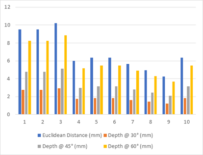
Figure 5 Bar chart
B. Validation
with Manual Measurements
To
further evaluate the accuracy of the proposed approach, additional validation
experiments were performed on a concrete specimen where both physical and
image-based crack width measurements were available. Manual crack widths were
recorded at marked intervals using a ruler, while the same crack was analyzed
using the proposed image-based method.
Figure 3
shows an annotated image of the crack where manual measurements (in cm) are
written beside the specimen, and the corresponding automated results (in mm) are
superimposed in red. The comparison demonstrates close agreement: for example,
a manual measurement of 0.3 cm corresponds to an automated result of
approximately 3 mm, while 0.5 cm corresponds to 5 mm.
To
further confirm calibration accuracy, a physical scale was placed directly
across the crack, as shown in Figure 6. This reference measurement illustrates
how the pixel-to-millimeter conversion factor was derived and validated. Using
the physical scale, the error between manual and automated measurements was
estimated to be within ±0.2 mm for crack width. Table 3 presents selected
comparison results, highlighting the consistency between manual and automated
measurements.
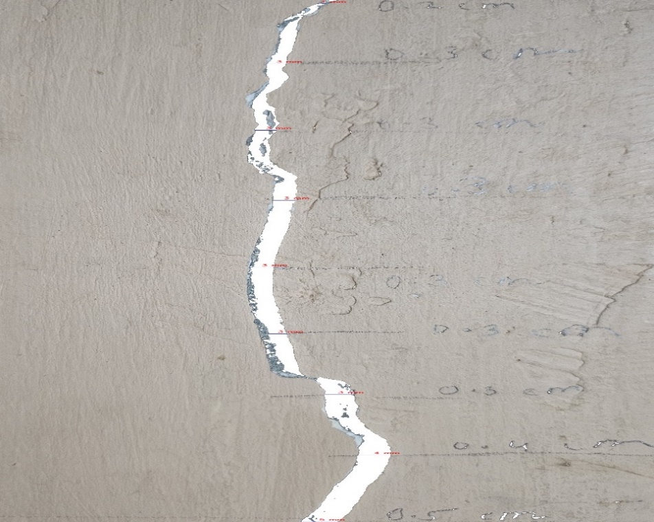
Figure 6 Crack
width validation: manual measurements (cm) versus automated results (mm)
These
results confirm that the proposed method produces measurements consistent with
independent manual readings, thereby reinforcing its accuracy and reliability.
While the validation was performed on a specimen different from that used in
the main experiments, it provides strong supporting evidence of the method’s
robustness.
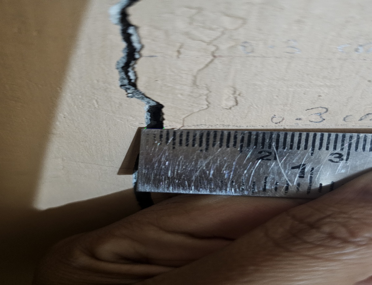
Figure 7 Manual
measurement of crack width using a physical ruler (scale in centimeters) for
calibration and validation of the pixel-to-millimeter conversion factor.
Table 3.
Comparison of manual and automated crack width measurements
|
Location
|
Manual Measurement (cm)
|
Manual Equivalent (mm)
|
Automated Measurement (mm)
|
Difference (mm)
|
|
Point 1
|
0.2 cm
|
2 mm
|
1 mm
|
1
|
|
Point 2
|
0.3 cm
|
3 mm
|
3 mm
|
0
|
|
Point 3
|
03 cm
|
3 mm
|
3 mm
|
0
|
|
Point 4
|
0.3 cm
|
3 mm
|
3 mm
|
0
|
|
Point 5
|
0.3 cm
|
3 mm
|
3 mm
|
0
|
|
Point 6
|
0.3 cm
|
3 mm
|
3 mm
|
0
|
|
Point 7
|
0.3 cm
|
3 mm
|
3 mm
|
0
|
|
Point 8
|
0.4 cm
|
4 mm
|
4 mm
|
0
|
|
Point 9
|
0.5 cm
|
5 mm
|
5 mm
|
0
|
C.
Error
Estimation (First Approximation)
Although
the proposed method demonstrates good agreement with manual crack width
measurements, it is also important to evaluate potential error sources. In this
study, two main sources of uncertainty are considered: (A) the conversion from
pixels to millimetres and (B) the assumption of a uniform crack slope (30°,
45°, 60°) for depth estimation.
A.
Pixel-to-Millimetre Conversion Error
The scale factor used in this study (e.g., 0.0909 mm/pixel, calibrated from the
ruler in Figure 7) converts pixel distances into real-world units. Small errors
in calibration or pixel localization propagate into width measurement errors.
For a measured crack width of 5 mm, the propagated width error is approximately
±0.1 mm (≈2%).
B.
Depth Estimation Error
Crack depth is derived from formula 9. Any uncertainty in measured width and
assumed slope propagates to depth error. Because the tangent function amplifies
slope variations, even a ±5° variation in the assumed crack angle can lead to
~18–20% relative error in depth estimation, whereas width error contributes
only ~1%.
The
methodology can be adapted for various use cases, including assessing
structural damage in buildings, evaluating surface cracks in materials, and
monitoring the integrity of infrastructure. Future work may include enhancing
the algorithm to detect and quantify more complex crack patterns, such as
branching cracks or cracks with irregular edges. Additionally, integrating
machine learning techniques could further automate the process and improve
accuracy in identifying and classifying different types of cracks.
This
crack quantification method provides a systematic approach for measuring crack
width and depth using image processing techniques, enabling detailed analysis
of crack characteristics for research and practical applications in material
science and engineering.
1. Choi, S., & Shah, S. P. (1997). Measurement of deformations on concrete specimens using image analysis. Experimental Mechanics, 37(3), 272–278. https://doi.org/10.1007/BF02317417
2. Duda, R. O., & Hart, P. E. (1972). Use of the Hough transformation to detect lines and curves in pictures. Communications of the ACM, 15(1), 11–15. https://doi.org/10.1145/361237.361242
3. Hutchinson, T. C., & Chen, Z. (2006). Improved image analysis for evaluating concrete damage. Journal of Computing in Civil Engineering, 20(3), 210–216. https://doi.org/10.1061/(ASCE)0887-3801(2006)20:3(210)
4. Li, Z., Yu, X., & He, W. (2018). Three-dimensional crack depth measurement for civil engineering applications using stereo imaging. Sensors, 18(3), 839. https://doi.org/10.3390/s18030839
5. Liu, S., & Sun, L. (2017). Application of digital image correlation for crack detection and quantification in concrete structures. Advances in Civil Engineering, 2017, Article ID 8023680. https://doi.org/10.1155/2017/8023680
6. Omar, M., El-Basyouny, N., Khattab, A., & El-Gizawy, M. (2018). Image-based crack detection in concrete structures using convolutional neural networks. Automation in Construction, 91, 116–130. https://doi.org/10.1016/j.autcon.2018.03.005
7. Otsu, N. (1979). A threshold selection method from gray-level histograms. IEEE Transactions on Systems, Man, and Cybernetics, 9(1), 62–66. https://doi.org/10.1109/TSMC.1979.4310076
8. Sahoo, P. K., Soltani, S., & Wong, A. K. C. (1988). A survey of thresholding techniques. Computer Vision, Graphics, and Image Processing, 41(2), 233–260. https://doi.org/10.1016/0734-189X(88)90022-9
9. Wang, X., Yang, Q., Wang, J., & Li, X. (2019). Crack width measurement based on image processing and adaptive Gaussian fitting. Measurement, 148, 106877. https://doi.org/10.1016/j.measurement.2019.106877
10. Yamaguchi, T., & Hashimoto, S. (2010). Fast crack detection method for large-size concrete surface images using percolation-based image processing. Machine Vision and Applications, 21(5), 797–809. https://doi.org/10.1007/s00138-009-0199-8
11. Zhang, Z., Li, Q., Mao, Z., & Shi, Z. (2020). A vision-based approach for automatic crack detection and quantification in concrete structures. Construction and Building Materials, 251, 118965. https://doi.org/10.1016/j.conbuildmat.2020.118965
12. Zou, Q., Zhang, L., Li, Q., Qi, X., Wang, Q., & Wang, S. (2019). DeepCrack: Learning hierarchical convolutional features for crack detection. IEEE Transactions on Image Processing, 28(3), 1498–1512. https://doi.org/10.1109/TIP.2018.2878966