Image processing and visualization tools
are an indispensable part during performing microsurgical endovascular
procedures with catheters on the heart. Existing visualization and image
processing methods limit the range of complex manipulations performed on the beating
heart. In its turn, classical visualization techniques (echocardiography,
fluoroscopy, and angiography) [1–3] possess several crucial disadvantages
such as insufficient quality of the output data, high level of noise and
limited scope (field of view). These drawbacks significantly reduce the range
of possible transcatheter procedures on the heart by means of endovascular
technology and also hinder the development of this area. Two-dimensional
echocardiography (EchoCG) does not allow adequately displaying the spatial
position of the medical instrument (catheter) and visualize the area of
interest. Additionally, 3D EchoCG displays a limited area with a significant
level of digital noise, shadows, and artifacts. Thus, for today, a wide range
of cardiosurgical operations are performed only on an open heart using
artificial circulation [4,5]. Such methods of pathology correction
have a number of shortcomings associated with severe postoperative
complications and long-term rehabilitation, which is an important problem in
cardiology. The availability of new methods of visualization, image processing
and delivering catheter devices allows performing a number of interventions on
the working heart, including stenting of vessels, radiofrequency ablation in
cases of cardiac arrhythmias, closing of atrial and interventricular septal
defects. Currently, there are a few numbers of research studies that are
devoted to the application of recognition and tracking of medical devices.
Nowadays biplane fluoroscopy that uses
X-ray image intensifier is one of the most frequently used methods of
visualization (up to 60%) [6]. In the studies of Matthias Hoffman, a
semi-automatic reconstruction of the catheter is performed based on two
projections [7,8]. The authors minimized the interaction
with the user in their algorithm; nevertheless, recognition still requires the assigning
of at least one point belonging to the catheter area. The accuracy of the
methods is at a high level, but the total processing time takes about 8 seconds,
which confirms the impossibility of using this method in real time. Moreover,
the X-ray based methods are not applicable for heart imaging, because they
cannot provide soft tissue information.
Research study on the skeletonization and
visualization of the catheter in the three-dimensional space of the vasculature
were carried out by Baert Shirley, Van de Kraats Everine and others [9]. Another research devoted to the
detection and tracking of different types of catheters was performed by Ying
Liang Ma et al. [10]. In their study, scientists did not
reconstruct the catheter but only used the tracking algorithm for three
different types of catheters.
In the other work, P. Ambrosini et al.
proposed a method, based on a hidden Markov model, for 3D catheter tip tracking
with 2D X-ray catheterization sequence and 3D rotational angiography [11]. But in the research intraoperative
images are enhanced using contrast agent for visualizing the vasculature.
In paper [12] the authors describe a
method based on registration X-rays and echocardiography. The presented algorithm had an average error of less than 1 mm and the
speed could reach 1.5 fps. However, the combination of X-rays and ultrasound
signals impose restrictions on the structure of input data end equipment. In
this regard, the main scientific direction of this study is the research and
development of the algorithm for intraoperative imaging and catheter
visualization using the 3D echocardiography data.
Epicardial full-volume 3D echocardiography
datasets were acquired on the porcine heart using an X7-2t transducer on a
Philips iE33 machine and PMS5.1 Ultrasound software (Philips Healthcare,
Andover MA). During the data acquisition step, 9 datasets were acquired. Each
dataset consists of 15-17 timeframes and each of them includes 208 slices of
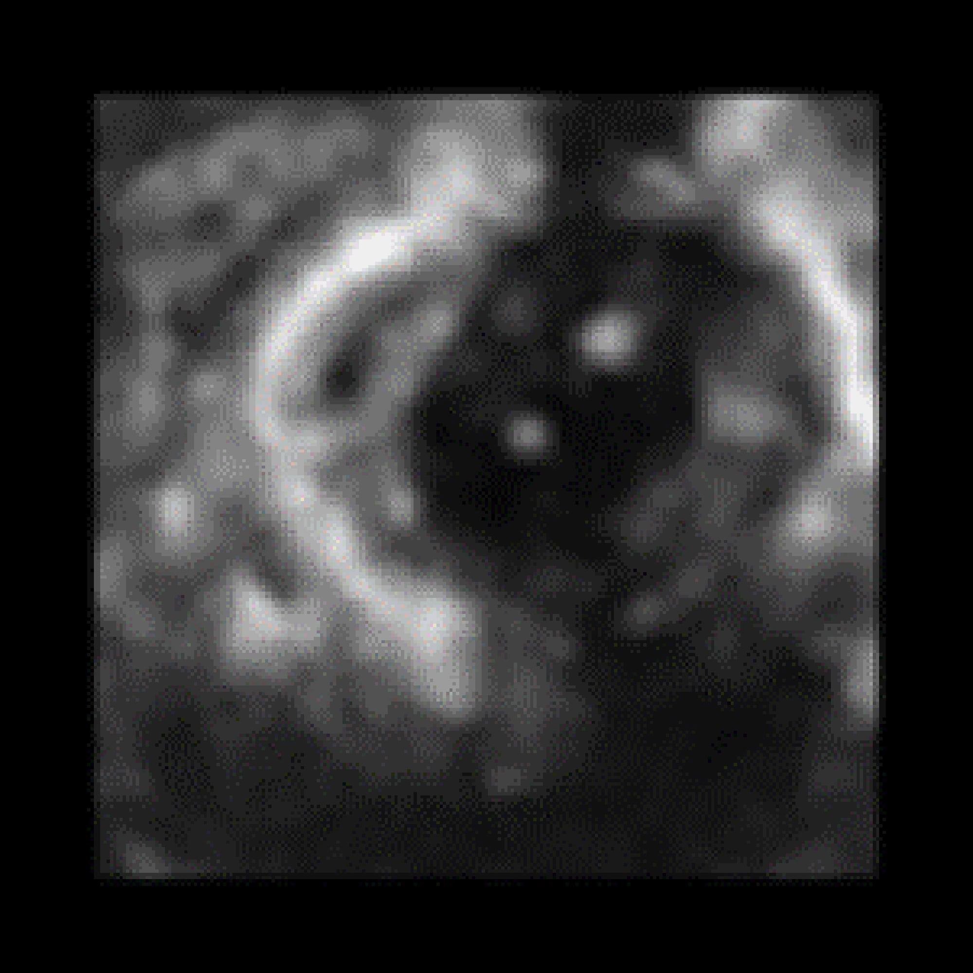
176*176-pixel size. Example of the data acquiring using Philips iE33 echocardiographer
is shown in Fig. 1.
The experimental protocols were approved by
the Boston Children’s Hospital Institutional Animal Care and Use Committee
(IACUC).
The datasets were processed offline on the
computer equipped with Intel Core i7-4790K 4.0 GHz CPU and NVIDIA GeForce 960
GT using MATLAB (MathWorks,
Natick MA).

Fig. 1. An exemplary slice of the data.
To efficiently recognize and segment the
catheter we used sequential steps with particular options and setting for each
of them. Features selected for the algorithm are the most relevant properties
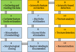
that can be used for the catheter recognition. The main steps of the algorithm
are presented as cascade-based workflow shown in Fig. 2.

Fig. 2. Basic steps for recognition and segmentation
algorithm of the catheter: green blocks – data acquisition and feature
studying, blue blocks – coarse detection and segmentation, orange blocks –
delicate detection and segmentation, red block – smoothed 3D reconstruction.
To gather the whole data, we used real-time
streaming of Philips iE33 machine. After getting all the medical data, we
transfer it from DICOM Philips format into Nearly Raw Raster Data (NRRD)
format.
In regard to the initial processing methods,
we applied automatic Otsu’s thresholding for binarization an image [13] and morphological closing based on morphological
reconstruction for filling the holes [14]. The disk-shaped element was used as
the main structuring element for this morphological procedure. Using a disk
structuring element allows preserving the circular nature of the object. In our
case, the catheter has the circular or elliptical shape depending on its
position and the position of the ultrasound transducer.
Small artifacts and noise emissions were
removed by the imposing area restrictions. The output of the previous
steps was a set of labeled regions including the region of interest (catheter).
However, among these regions, there are false ones (see Fig. 4b).
We put forward a hypothesis that, by
imposing different feature constraints, the catheter can be accurately found in
the image. We selected several high-impact features such as ROI area, mean and
standard deviation of intensity within a region and four textural features such
as contrast, correlation, energy, and homogeneity. In order to limit the number
of obtained regions, we calculated values of all features and entered limits
for them, which are equal to ranges, corresponding to the region of the
catheter. Textural features were calculated using gray-level co-occurrence
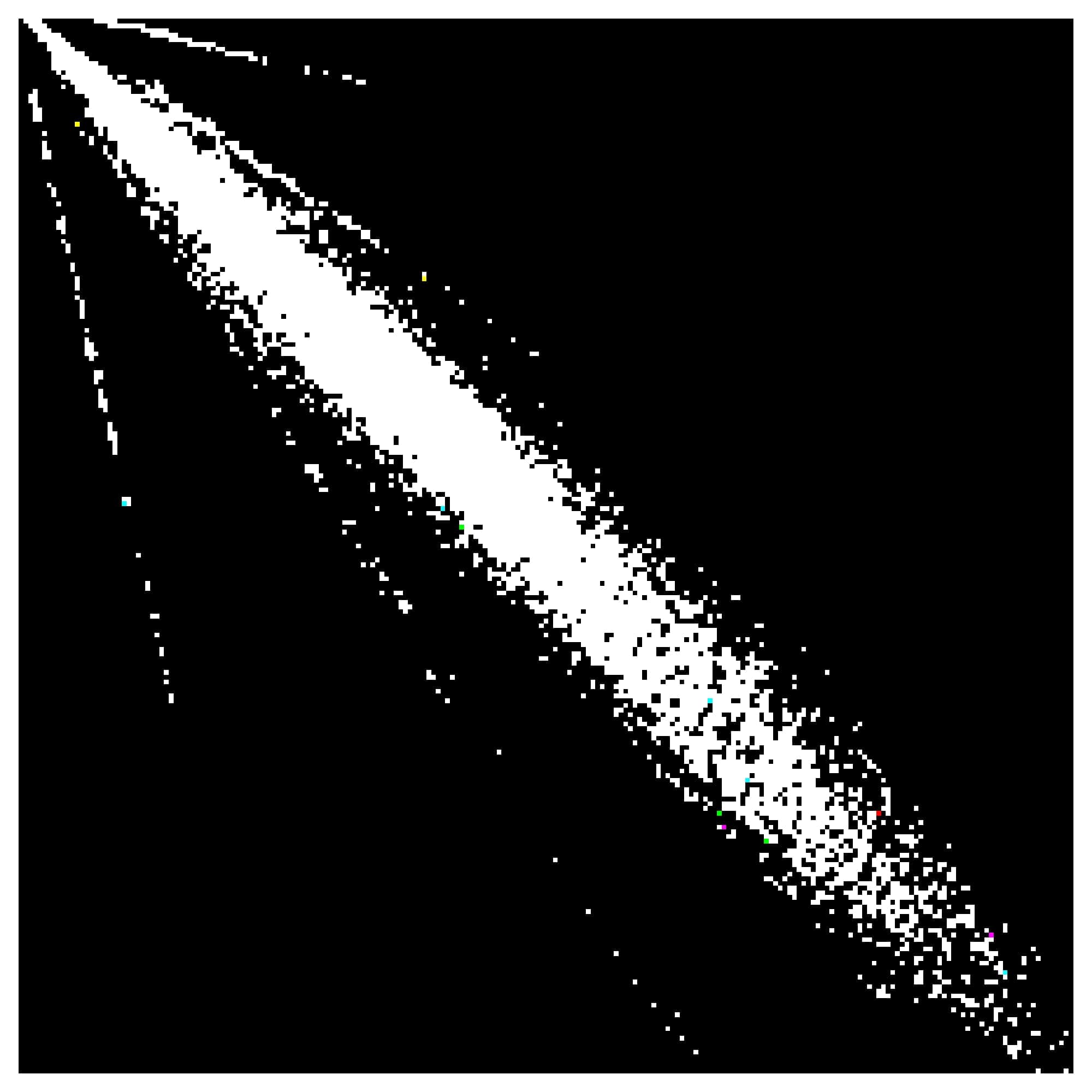
matrix (GLCM) [15,16]. The GLCM for an exemplary slice is
shown in Fig. 3.

Fig. 3. GLCM for an exemplary slice.
In order to compute textural features, GLCM
should be normalized, so that the sum of its elements is equal to 1. Each
element (r,c) in the normalized GLCM is the joint probability occurrence
of pixel pairs with a defined spatial relationship having gray level values r
and c in the image.
Statistical properties of the image derived
from GLCM are following:
Contrast is a measure of the intensity
variance or inertia between a pixel and its neighbor over the whole image.
Contrast range for GLCMs (255*255 size) is from 0 to 64516. For the constant image,
contrast is equal to 0. Contrast is calculated as follows:

1.
Correlation
is a measure of how correlated a pixel is to its neighbor over the whole image.
Correlation varies from 1 to -1. Perfectly positively or negatively correlated
image corresponds to 1 or -1 for correlation. Correlation is calculated as
follows:

2.
Energy
is the sum of squared elements in the GLCM and it ranges from 0 to 1. Energy is
calculated as follows:

3.
Homogeneity
is a value that measures the closeness of the distribution of elements in the
GLCM to the GLCM diagonal.

where:
p(i, j) is an element (i, j) of the
normalized symmetrical GLCM;
N is the number
of gray levels;
µ is the GLCM
mean (being an estimate of the intensity of all pixels in the relationships
that contributed to the GLCM), calculated as follows:

σ is the
variance of intensities of all reference pixels in the relationships that contributed
to the GLCM, calculated as:

Most regions similar to the region of the
catheter were excluded after application delicate detection based on texture
features and Gray-Level Co-Occurrence Matrix. It should also be noted, that
threshold levels for textural and intensity features were empirically found.
The GLCM is a widely used technique, which
is applied not only to the feature extraction but also for segmentation tasks.
For instance, A. Rampun, H. Strange et al. proposed a segmentation method based
on consideration each feature at two different configurations in the paper [17]. Mahesh B. Nagarajan, Markus B. Huber
et al. used the GLCM for the lesion segmentation in the work [18].
After acquiring the data and figuring out
the catheter feature distribution, each slice is processed by the automatic
thresholding algorithm. The result of the application of Otsu’s thresholding
method is shown in Fig. 4a.
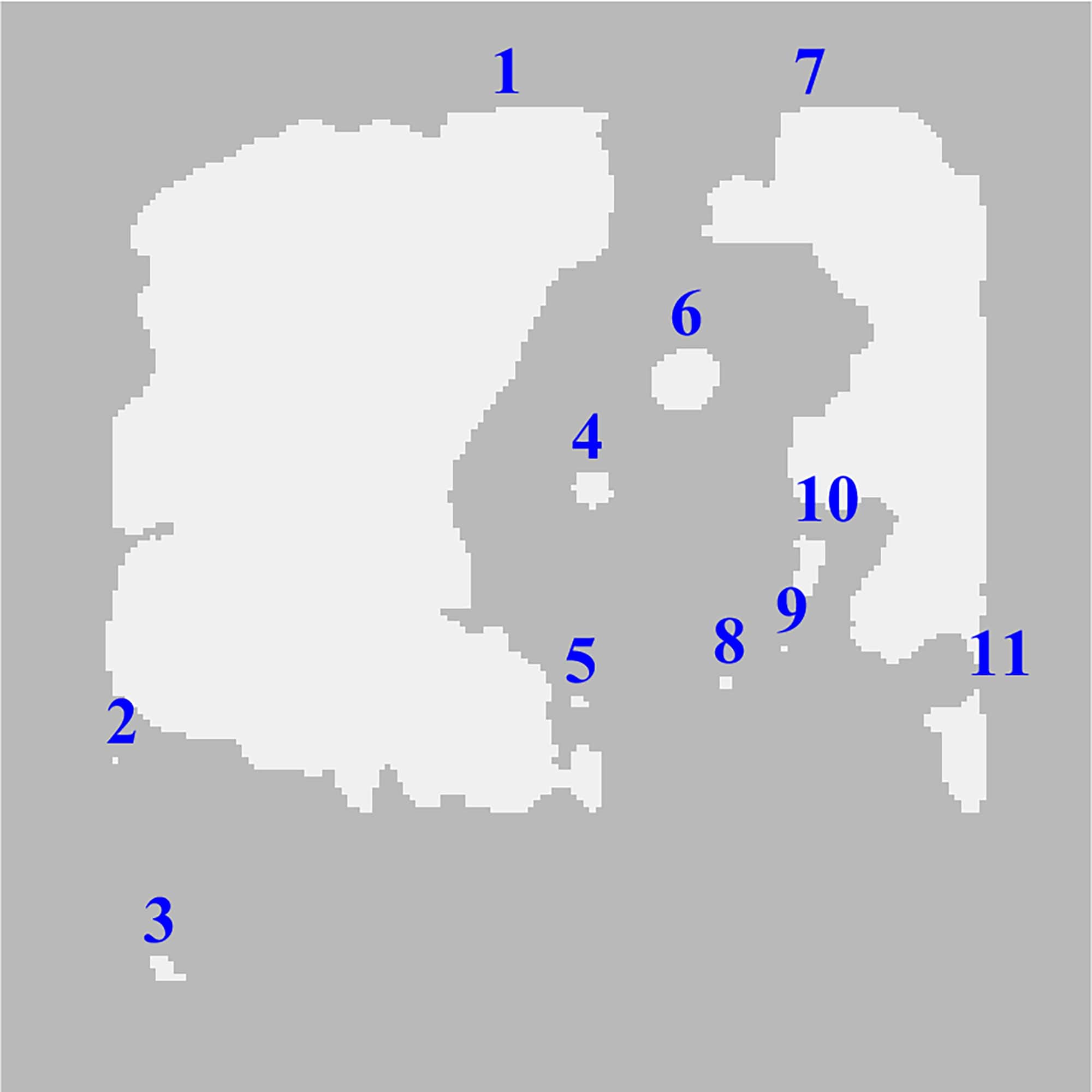
The morphological
closing follows the thresholding step and performs a flood-fill operation on
background pixels (see Fig. 4b). This operation fills the holes and
determines the connected area. At this step, we used 4-connected neighborhoods
connectivity. As it can be seen in Fig. 4b, the number of objects of these
steps is 11, where the catheter is represented by the region 6.
Fig. 4. Automatic thresholding (a) and flood-fill
segmentation (b).
As we described above, one of the workflow
steps is an intermediate procedure connected with excess blobs elimination.
This step assumes that the region of the catheter cannot be smaller than 5 pixels
even for an edged slice of the distal end of the catheter. This is why regions
2 and 9 reflected in Fig. 4b and shown in Fig. 5a in red circles were removed. The
output of this step is a black and white (BW) mask with 9 objects.
Fig. 5. Excess blobs elimination: colorized input (a) and
BW output (b).
As illustrated in Fig. 6 most regions are removed after step 7
of the workflow but there are 4 excess regions that meet the area criteria as
well as the region of the catheter.

Fig. 6. Exclusion of the regions by area criteria.
After finishing the coarse detection and
segmentation, we apply intensity analysis with further segmentation using the
features. The first two features related to this step are the intensity mean
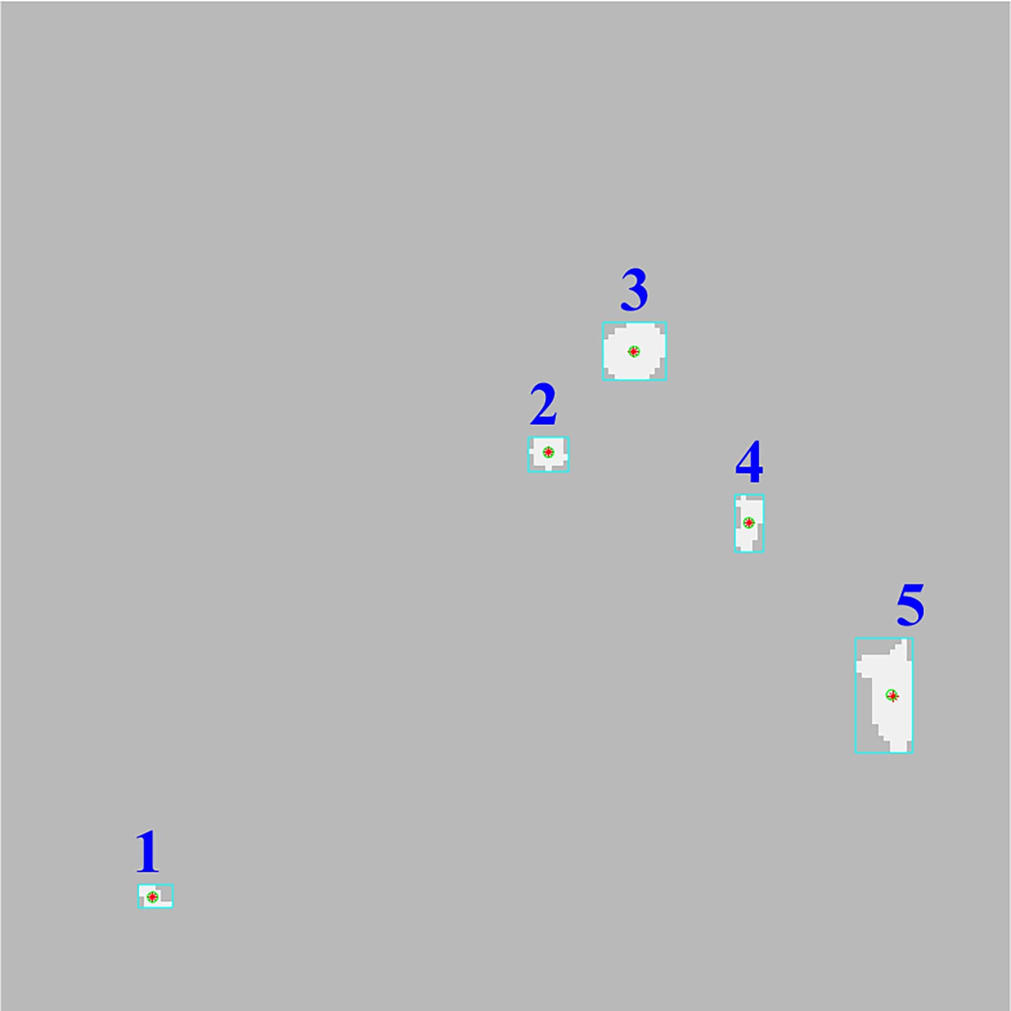
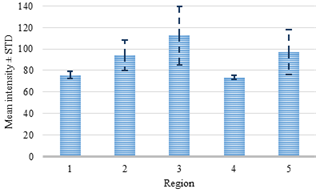
and standard deviation of a certain region. To detect the region of the
catheter, the mean and standard deviation were computed for each region on each
slice of the dataset. The distribution of these two features for the current
slice is presented in Fig. 7, where the average intensity and
standard deviation for the catheter are 112 and 27, respectively. In its turn,
several regions significantly differ from the region of the catheter, for
example, region 1 and 4. In this regard, the obvious difference between the two
classes (tissue and catheter) allowed linear SVM to set a threshold value for
the features.

Fig. 7. Intensity analysis for the regions.
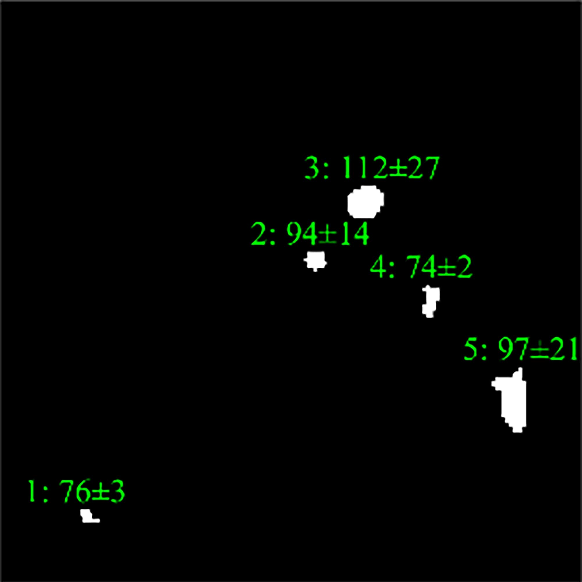
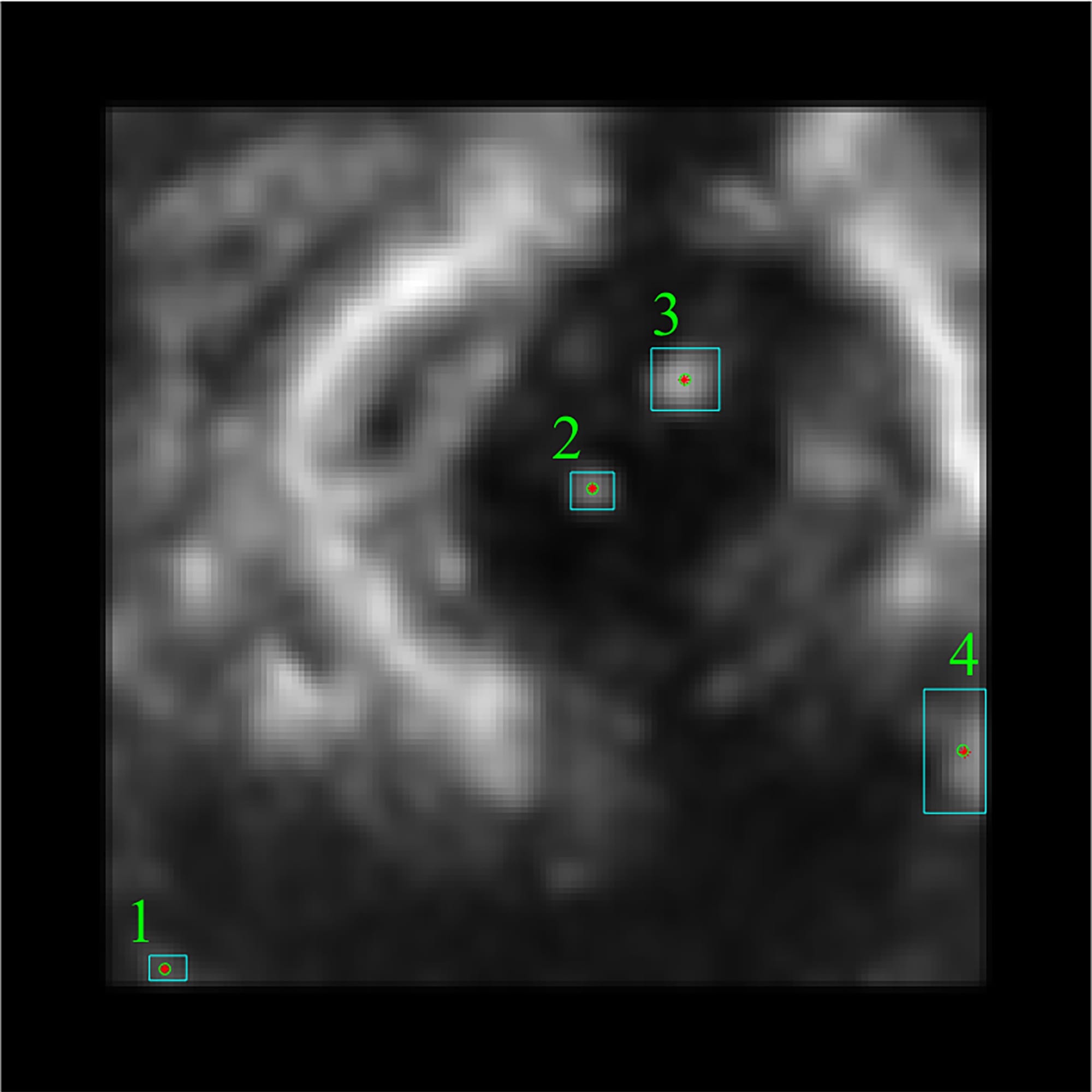
Values of these features for each region
are compared to limits and are defined whether they meet the criteria or not. Fig. 8 displays how these two features
excluded one of the redundant regions.
|

|

|
|
a)
|
b)
|
Fig. 8. Intensity analysis (a) with the following
intensity-based detection using mean and standard deviation (b).
The most precise step of the workflow is
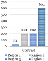
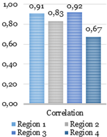
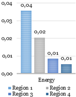
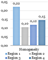
texture analysis with the GLCM. During this stage, four parameters such as the contrast,
homogeneity, correlation, and energy are computed using GLCMs of each region.
Four GLCMs for remained regions are shown
in Fig. 9. Afterward, textural
features were compared with established limits. Computed feature values of the
texture analysis shown below in Fig. 10 were compared to the reference ones shown
in Fig. 12.
|

|

|
|
Region 1
a)
|
Region 2
b)
|
|

|

|
|
Region 3 (catheter)
c)
|
Region 4
d)
|
Fig. 9. Visual representation of GLCMs for remained
regions.
The catheter
(region 3) and two other regions (region 1 and 2) in Fig. 10 have sufficient uniformity, as
indicated by the arrangement of the matrix elements on the central diagonal. In
turn, the region 4 has internal brightness differences. Since the GLCM
uniformity of the region cannot be used as a feature of the catheter. The correlation,
contrast, homogeneity, and energy were computed based on the obtained data.
Further processing was performed on the obtained features.
Fig. 10. Texture analysis: contrast (a), correlation (b),
energy (c) and homogeneity (d).
The final procedure of the 2D stage found
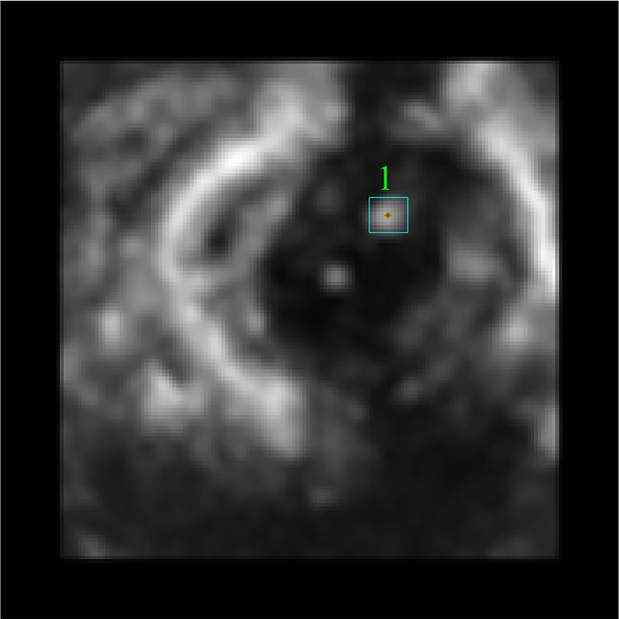
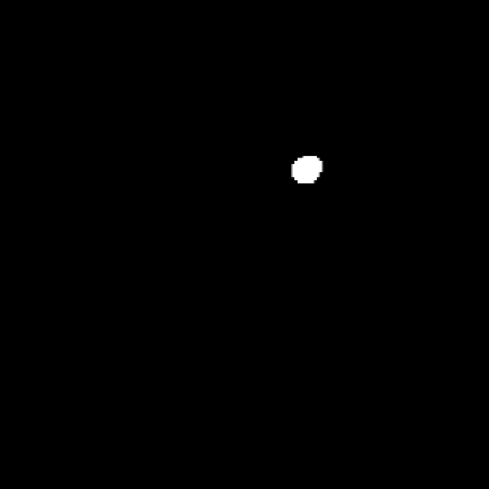
the desired ROI with certain features (see Fig. 11). As it can be seen in Fig. 11b, this step leaves only the region of the catheter and gives
the output as a black and white mask which can be used for further 3D
reconstruction.
|

|

|
|
a)
|
b)
|
Fig. 11. A detected catheter (a) and its BW mask (b).
In order to
eliminate blobs and leave the desired region of interest (ROI), we imposed
general area limitations performed in the beginning: the lowest and highest area
limits are 5 and 200 pixels respectively. We also performed an estimation of
feature limits within one timeframe consisting of 208 slices in order to find
out the distribution of lowest and highest values for further restriction. This
number of slices is sufficient to MsoNormal out the feature distribution because
all settings for the data acquisition were not changed within the study. In
this regard, other 3D timeframes have relatively the same feature distribution.
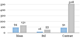
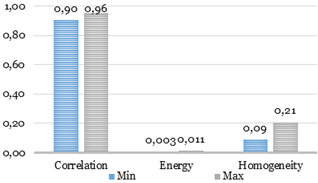
Feature limits obtained with 208 slices are shown in Fig. 12.
One of the main limitations of the
algorithm is area restriction. Many excess binary large objects (blobs)
frequently remain after application thresholding.


Fig. 12. Feature limits for the catheter.
To assess the accuracy of the algorithm, we compared two diameters: the
reference diameter and the diameter received after the application of the
proposed algorithm. The catheter used for performing medical procedures in our
case had a diameter equal to 7 Fr (French Gauge) or 2.333 mm.
The diameter of the catheter was estimated
using 2 ways: manual and automatic. For manual measurements, we used the short-axis
view. Using this view gives a bigger sample of measurements what makes
calculations of the diameter with higher precision.
However, these measurements can be taken in the long-axis view but with lower
accuracy. To assess the accuracy, the diameter was measured in 504 slices. To
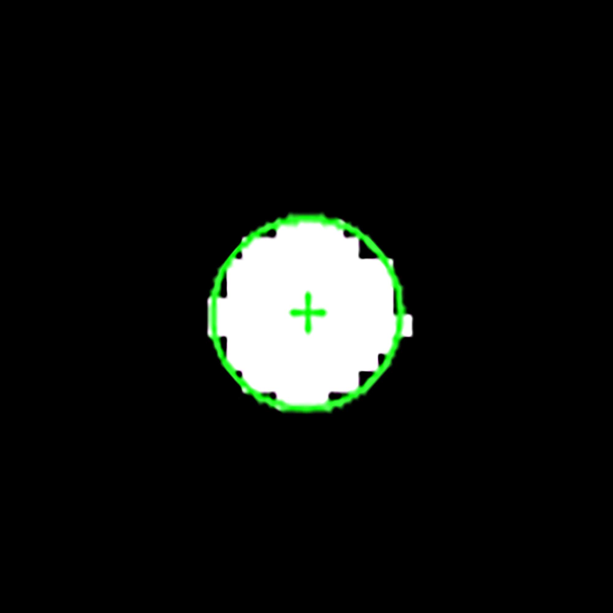
gauge the diameter automatically, we described the region of the catheter by
the corresponding ellipse that has the same second moment (see Fig. 13).

Fig. 13. Zoomed mask of the catheter region with an ellipse
replacement.
As it can be seen in Table 1, the average diameter of the
catheter after executing all processing steps equals to 2.47 mm what is 5.84%
more than the reference diameter. However, such error does not have a strong
influence on the visualization because 0.14 mm error lets a surgeon perform
medical procedures without any confusions. It was observed that Otsu’s
thresholding method incrassates the region of the catheter by 5-10% this is why
the error is increased as well. To decrease the error, modified Otsu’s method
and/or more delicate threshold level should be used. It’s important to note
that accuracy measurement performed by the algorithm took into account position
and inclination of the catheter, which allowed better orientation along the
correct axes.
Table 1. Comparison of the reference catheter diameter with the diameter obtained
by the proposed algorithm.
|
|
Reference
diameter
|
Diameter measured by the
algorithm
|
|
Mean,
mm
|
2.33
|
2.47
|
|
Std,
mm
|
0
|
0.16
|
|
Error,
%
|
0
|
5.84
|
A reduction tendency of a number of regions
over different steps of the proposed algorithm is shown in Table 2. According to the results, there is a
trend of decreasing the number of regions. The intensity-based and area-based
features reduced the number of regions approximately by half. In turn, texture
feature based on the GLCM allowed excluding the false regions more accurately.
Speaking of recognition accuracy and several mathematical statistics, they are shown
in Table 3. The average
recognition accuracy of the catheter is 87.2%. The confidence
level for the sample including 504 cases equals 2.5%. The latter means that the
recognition accuracy varies from 84.6% to 89.7% with a 5% significance level.
Table
2. A number of regions within different
steps of the proposed algorithm.
|
Number
of regions
|
Mean±STD
|
|
Initial number of
regions
|
10.1±3.4
|
|
Number
of false regions
|
9.1±3.4
|
|
Number
of regions after area restriction (low limit)
|
8.9±3.2
|
|
Number
of regions after area restriction (high limit)
|
6.7±2.9
|
|
Number
of regions after intensity restriction
|
5.5±2.5
|
|
Number
of regions after texture restriction
|
1.2±0.3
|
Table
3. Mathematical statistics and recognition
accuracy.
|
Parameter
|
Value
|
|
Significance level
|
0.05
|
|
Size
|
504
|
|
Confidence interval
|
2.5%
|
|
Recognition accuracy
|
87.2%
|
The desktop computer with equipment
described in section 2.1 was
used for time assessment. We did not isolate the testing process from the
influence of other processes and did not allocate a separate thread. To find
the mean and standard deviation of processing time we performed 150-iteration
assessment. Processing time for one timeframe is 1.96±0.045 seconds. Each
timeframe includes 208 slices what means that average processing time for
176*176 slice is 9±0.2 milliseconds.
In this research study, we developed an
image-based algorithm detecting and tracking the distal end of the catheter. To
correctly detect and segment the catheter, we applied a feature-based approach
that can recognize the catheter along the whole 3D dataset. However, the
algorithm works in pseudo-3D what means that it processes the data in the slice-by-slice
mode. It worth noticing that the accuracy of the algorithm is at the relatively
high level and equal to 94.16%. This means that the algorithm error is 140
micrometers. However, this error is acceptable for performing
minimally-invasive cardiac surgery. Another vital feature of the algorithm is
its processing time. Average processing time for one 3D timeframe is equal to
1.96 seconds and approximately 9 milliseconds per slice. Though the algorithm
is not time-consuming, it is still complicated to apply it to real-time surgery
because of the huge amount of data obtained by echocardiography.
This work was supported in part by the
Russian Federation Governmental Program “Nauka” № 12.8205.2017/БЧ (addition
number: 4.1769.ГЗБ.2017). The experimental calculations are carried out at
Tomsk Polytechnic University within the framework of Tomsk Polytechnic
University Competitiveness Enhancement Program grant.
1. Luani B. et al. Zero-fluoroscopy cryothermal
ablation of atrioventricular nodal re-entry tachycardia guided by endovascular
and endocardial catheter visualization using intracardiac echocardiography //
J. Cardiovasc. Electrophysiol. 2018. Vol. 29, № 1. P. 160–166.
2. Schwein A. et al. Computed tomography
angiography-fluoroscopy image fusion allows visceral vessel cannulation without
angiography during fenestrated endovascular aneurysm repair // J. Vasc. Surg.
2018.
3. Cheung N.K. et al. Radiation exposure, and
procedure and fluoroscopy times in endovascular treatment of intracranial
aneurysms: a methodological comparison // J. Neurointerv. Surg. 2018. P. neurintsurg-2017-013596.
4. Spitzer E. et al. The Role of Automated 3D
Echocardiography for Left Ventricular Ejection Fraction Assessment // Card. Fail.
Rev. 2017. Vol. 3, № 2. P. 97.
5. Muraru D. et al. Three-dimensional speckle-tracking
echocardiography: benefits and limitations of integrating myocardial mechanics
with three-dimensional imaging // Cardiovasc. Diagn. Ther. 2018. Vol. 8, № 1.
P. 101–117.
6. Tepeler A. et al. Factors affecting the
fluoroscopic screening time during percutaneous nephrolithotomy // J Endourol.
2009. Vol. 23, № 11. P. 1825–1829.
7. Hoffmann M. et al. Semi-automatic catheter
reconstruction from two views. // Med. image Comput. Comput. Interv. 2012. Vol.
15, № Pt 2. P. 584–591.
8. Hoffmann M. et al. Electrophysiology catheter
detection and reconstruction from two views in fluoroscopic images // IEEE
Trans. Med. Imaging. 2016. Vol. 35, № 2. P. 567–579.
9. Baert S.A.M. et al. Three-Dimensional Guide-Wire
Reconstruction from Biplane Image Sequences for Integrated Display in 3-D
Vasculature // IEEE Trans. Med. Imaging. 2003. Vol. 22, № 10. P. 1252–1258.
10. Ma Y. et al. Real-time x-ray fluoroscopy-based
catheter detection and tracking for cardiac electrophysiology interventions. //
Med. Phys. 2013. Vol. 40, № 7. P. 071902.
11. Ambrosini P. et al. A Hidden Markov Model for 3D
Catheter Tip Tracking with 2D X-ray Catheterization Sequence and 3D Rotational
Angiography // IEEE Trans. Med. Imaging. 2017. Vol. 36, № 3. P. 757–768.
12. Wu X. et al. Catheter tracking in 3D
echocardiographic sequences based on tracking in 2D X-ray sequences for cardiac
catheterization interventions // Proceedings - International Symposium on
Biomedical Imaging. 2013.
13. Otsu N. A Threshold Selection Method from Gray-Level
Histograms // IEEE Trans. Syst. Man. Cybern. 1979. Vol. 9, № 1. P. 62–66.
14. Soille P. Morphological Image Analysis. Berlin,
Heidelberg: Springer Berlin Heidelberg, 2004. 392 p.
15. Haralick R.M., Shapiro L.G. Computer and Robot
Vision // Computer and Robot Vision. 1992. Vol. 1. 28-48 p.
16. Haralick R.M., Shanmugam K., Dinstein I. Textural
Features for Image Classification // IEEE Trans. Syst. Man. Cybern. 1973. Vol.
SMC-3, № 6. P. 610–621.
17. Rampun A., Strange H., Zwiggelaar R. Texture
segmentation using different orientations of GLCM features // Proceedings of
the 6th International Conference on Computer Vision / Computer Graphics
Collaboration Techniques and Applications - MIRAGE ’13. 2013.
18. Nagarajan M.B. et al. Classification of small
lesions in dynamic breast MRI: eliminating the need for precise lesion
segmentation through spatio-temporal analysis of contrast enhancement // Mach.
Vis. Appl. 2013. Vol. 24, № 7. P. 1371–1381.

