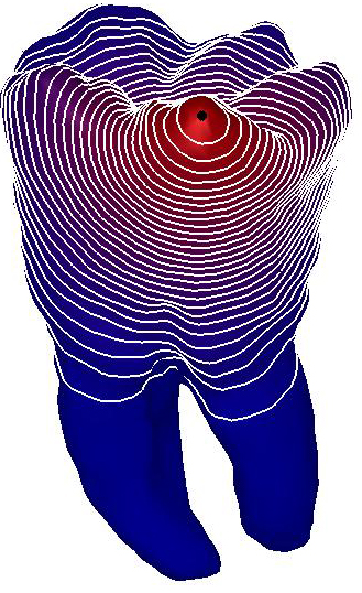
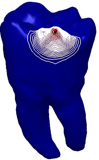
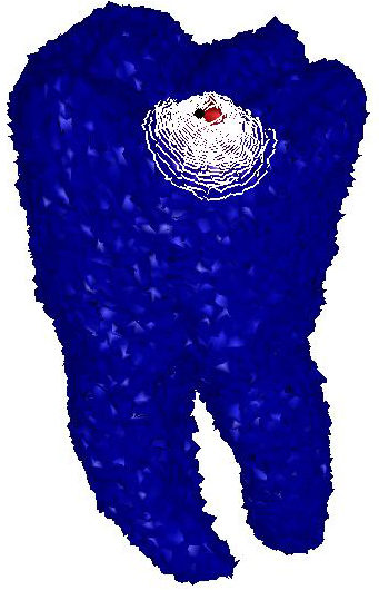
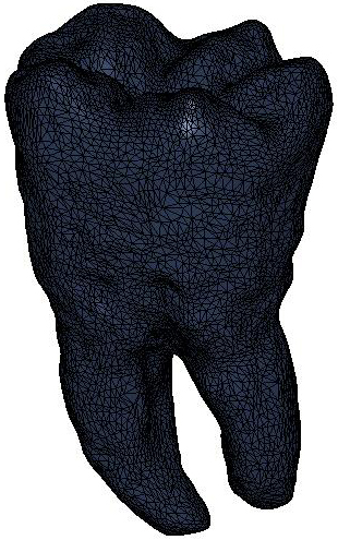
In medical applications, the heat kernel is
central in diffusion filtering and smoothing of images [1-6], 3D shapes [7, 8],
and anatomical surfaces [9, 10]. However, the computational cost for the
evaluation of the heat kernel is the main bottleneck for processing both
surfaces and volumetric data; in fact, it takes from O(n) to O(n3) time on a
data set sampled with n points, according to the sparsity of the Laplacian
matrix. This aspect becomes more evident for medical data, which are nowadays
acquired by PET, MRI systems and whose resolution is constantly increasing with
the improvement of the underlying imaging protocols and hardware.
To overcome the time-consuming computation
of the Laplacian spectrum on large data sets (Sect. 2), the heat kernel has
been approximated by prolongating its values evaluated on a sub-sampling of the
input surface [11-13]; applying multi-resolution decompositions [14] or a
rational approximation of the exponential representation of the heat kernel
[15]; and considering the contribution of the eigenvectors related to smaller
eigenvalues. The heat equation has been solved through explicit [16] or
backward [17, 18] Euler methods, whose solution no more satisfies the diffusion
problem. Further approaches apply a Krylov subspace projection [19], which
becomes computationally expensive when the dimension of the Krylov space
increases, still remaining much lower than n.
|

|

|
|
(a)
|
(b)
|
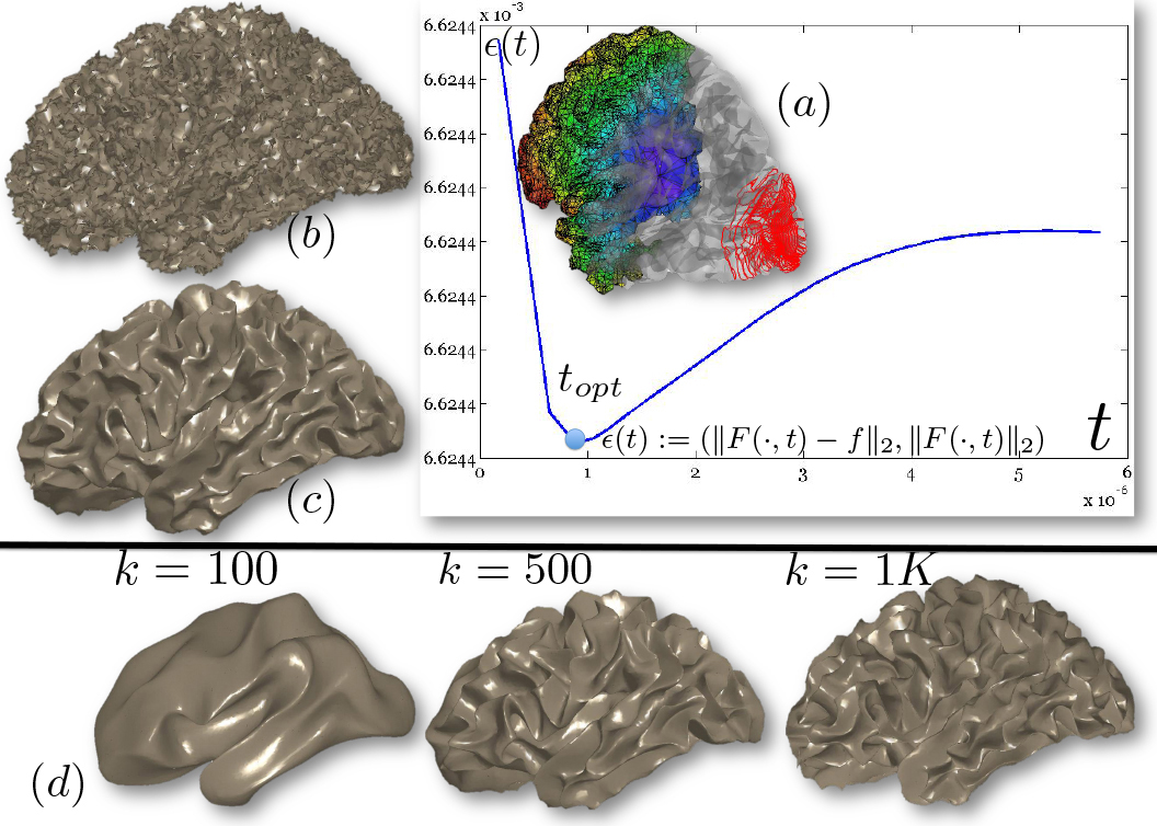
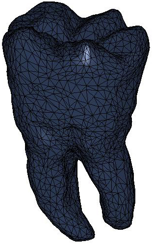
Figure
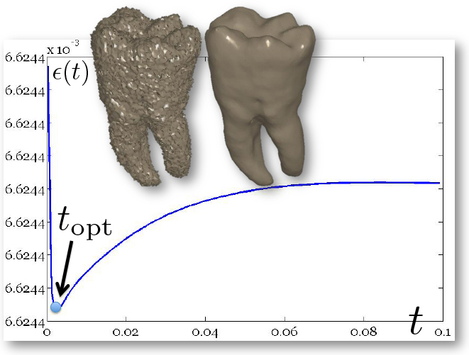
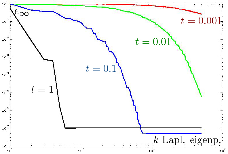
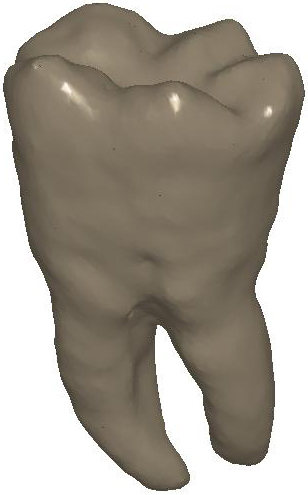
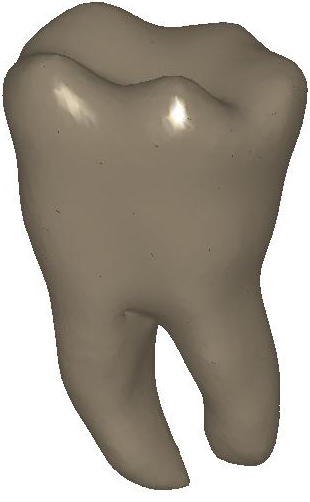
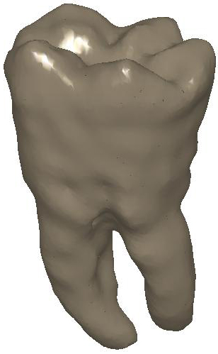
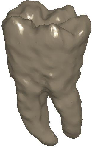
1: L-curve and ℓ∞
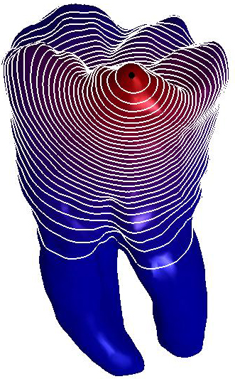
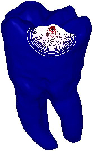
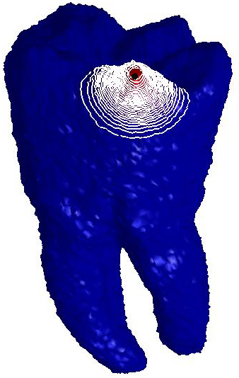
discrepancy. (a) Optimal parameter and
corresponding diffusion smoothing (upper part,
right−Padé-Chebyshev approximation of degree r=7) on the noisy 3D
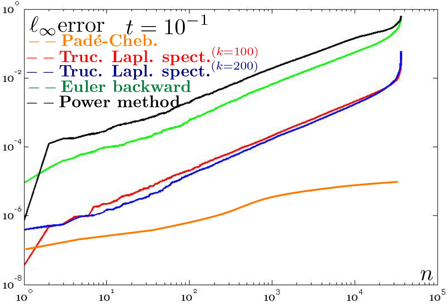
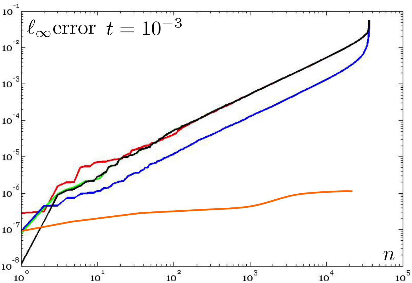
shapes of the teeth. (b) Error  (y-axis) between the Padé-Chebyshev approximation (r:=7) of
  and its truncated spectral approximation
  with k eigenpairs (k≤103, x-axis), and different values of
t.
This paper proposes an accurate,
computationally efficient, and spectrum-free evaluation of the diffusive smoothing
on 3D shapes, represented as polygonal meshes. The idea behind our approach
(Sect. 3) is to apply
the (r,r)-degree Padé-Chebyshev rational polynomial approximation
of the exponential map to the solution of the heat equation. This spectrum-free
formulation converts the heat equation to a set of sparse, symmetric linear
systems and the resulting computational scheme is independent of the evaluation
of the Laplacian spectrum, the selection of a specific subset of eigenpairs,
and multi-resolutive prolongation operators. Our approach has a linear
computational cost, is free of user-defined parameters, and works with sparse,
symmetric, well-conditioned matrices. Since the computation is mainly based on
numerical linear algebra, our method can be applied to any class of Laplacian
weights and any data representation (e.g., 3D shapes, multi-dimensional data),
thus overcoming the ambiguous definition of multi-resolutive and prolongation
operators on point-sampled or non-manifold surfaces. Bypassing the computation
of the eigenvectors related to small eigenvalues, which are necessary to
correctly recover local features of the input shape or signal, the
spectrum-free computation is robust with respect to data discretization. As a
result, it properly encodes local and global features of the input data in the
heat diffusion kernel. For any data representation and Laplacian weights, the
accuracy of the heat smoothing computed through the Padé-Chebyshev
approximation is lower than 10-r, where r:=5,7 is the degree of the
rational polynomial, and can be further reduced by slightly increasing r.
Finally (Sect. 4), our
experiments on surfaces and volumes representing anatomical data show that the spectrum-free
approach greatly reduces the computational cost (from 32 up to 164
times) and guarantee a higher approximation accuracy than previous work.
Let us consider the heat equation  , on a closed, connected manifold
  of
of  , where
  defines the initial condition on
  . The solution to the heat equation
  , is computed as the convolution
  between the initial condition f and the heat kernel
  . Here,
  is the Laplacian eigensystem
  .
.
|

|

|

|
|
(a)
|
(b)
|
(c)
|
|

|

|

|
|
(d) k=100
|
k=500
|
k=1K
|
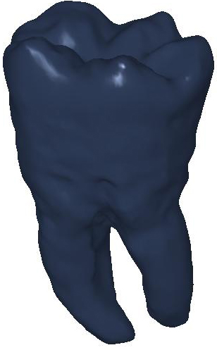
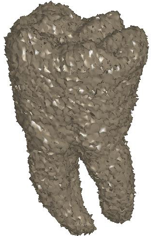
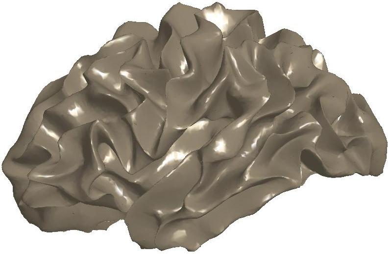
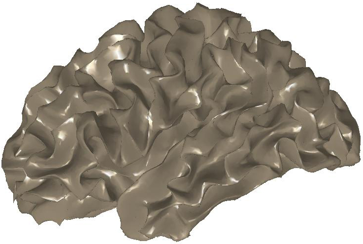
Figure
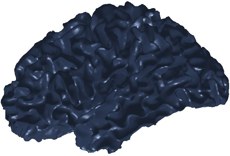
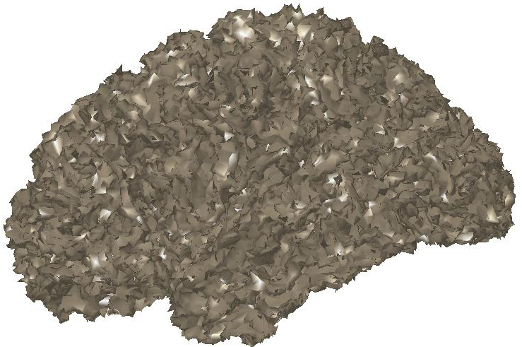
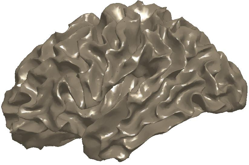
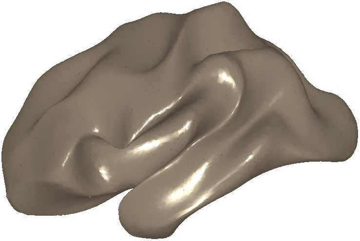
2: (a) Input and (b) noisy data set.
Diffusion smoothing of (b) computed with (c) the Padé-Chebyshev
approximation of degree r=7 and (d) the truncated approximation with k
Laplacian eigenparis. A low number of eigenpairs oversmooth the shape details;
increasing k reconstructs the surface noise. The ℓ∞
error between (a) and the smooth approximation of (b) is lower than 1% for (c)
the Padé-Chebyshev method and (d) varies from 12% (k=100) up to 13%
(k=1K) for the truncated spectral approximation.
The heat equation is solved through its FEM
formulation [20] on a discrete surface  (e.g., triangle mesh, point set) of
  . Indicating with
  the Laplacian matrix, which discretizes the Laplace-Beltrami
operator on
  , the “power” method applies the identity
  , where m is chosen in such a way that t/m is sufficiently small to
guarantee that the approximation
  is accurate. Here, I is the identity matrix. However, the selection
of m and its effect on the approximation accuracy cannot be estimated a-priori.
In [17, 18], the solution to the heat equation is computed through the Euler
backward method
  ,
,  . The resulting functions are over-smoothed and converge to a constant
map, as k→+∞. Krylov subspace projection [19], which replaces the Laplacian
matrix with a full coefficient matrix of smaller size, has computational and
memory bottlenecks when the dimension k of the Krylov space increases, still
remaining much lower than n (e.g., k≈5K).
|

|

|

|
|
(a)
|
(b)
|
(c)
|
|

|

|

|
|
(d) k=100
|
k=500
|
k=1K
|
Figure
3: (a) Input and (b) noisy data
set. Diffusion smoothing computed with (c) the Padé-Chebyshev
approximation and (d) the truncated approximation with k Laplacian
eigenparis. The truncated spectral approximation does not preserve sharp
features of the brain structure, which are accurately reconstructed by the
Padé-Chebyshev method.
Once the Laplacian matrix has been
computed, we evaluate its spectrum and approximate the heat kernel by
considering the contribution of the Laplacian eigenvectors related to smaller
eigenvalues, which are computed in superlinear time [21]. Such an approximation
is accurate only if the exponential filter decays fast (e.g., large values of
time). Otherwise, a lager number of eigenpairs is needed and the resulting
computational cost varies from O(kn2) to O(n3) time, according to the sparsity
of the Laplacian matrix. Furthermore, the number of eigenpairs is heuristically
selected and its effect on the resulting approximation accuracy cannot be
estimated without computing the whole spectrum. Finally, we can apply
multi-resolution prolongation operators [13] and numerical schemes based on the
Padé-Chebyschev polynomial [15, 22]. However, previous work has not
addressed this extension, convergence results, and the selection of the optimal
scale.

Figure
4: Heat diffusion smoothing of
noisy data with the Padé-Cebyshev and truncated spectral approximation.
(a) Input data set, represented as a triangle mesh, and L-curve of the
approximation accuracy (y-axis) versus the solution smoothness (x-axis). (b)
Data set achieved by adding a Gaussian noise to (a). Diffusion smoothing
computed with (c) the Padé-Chebyshev approximation of degree r=7 and (d)
the truncated approximation with k Laplacian eigenparis. A low number of
eigenpairs smooths local details; increasing k reconstructs the noisy
component. The ℓ∞ error between the ground-truth (a) and the
smooth approximation of (b) is lower than 1% for the Padé-Chebyshev
method (c) and varies from 12% (k=100) up to 13% (k=1K) for the truncated
spectral approximation (d).
Let us discretize the input shape as a
triangle mesh  , with vertices
  , which is the output of a 3D scanning device or a segmentation of a
MRI acquisition of an anatomical structure. Let
  be the Laplacian matrix, where
  is a symmetric, positive semi-definite matrix and
  is a symmetric and positive definite matrix. On triangle meshes,
  is the Laplacian matrix with cotangent weights [23, 24] or
associated to the Gaussian kernel [25], and B is the mass matrix of the Voronoi
[18] or triangle [26] areas. For any class of weights, the Laplacian matrix
  is uniquely defined by the couple (
 ,
, ) and is associated to the generalized eigensystem (X,Λ) such
that

where X and Λ are the eigenvectors’
and eigenvalues’ matrices. From the relation (1), we get the identities 

Then, the spectral representation of the
heat kernel is

For a signal  , sampled at
  , the solution
  , to the heat equation
  , is achieved by multiplying the heat kernel matrix
  with the initial condition
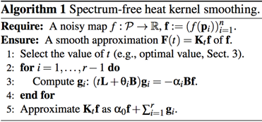
  . Applying the Padé-Chebyshev approximation to the
exponential of the Laplacian matrix in Eq. (3), we get

and the vector  is the sum of the solutions of r sparse linear systems

We briefly recall that the weights  and nodes
  of the Padé-Chebyshev approximation (4) are precomputed for
any polynomial degree [27]. Each vector gi is
calculated as a minimum norm residual solution [28], without pre-factorizing
the matrices L and B. Algorithm 1 summarizes the main steps of
the proposed computation.
|
Input
|
Surface Sampling
|
Noise
|
|
|
t=0.1
|
t=0.01
|
t=0.01
|

|

|

|

|
|
5K
|
|
|
|

|

|

|

|
|
20K
|
|
|
|
Figure
5: Robustness of the
Padé-Chebyshev approximation of the heat kernel with different values of
the time parameter and with respect to surface sampling and noise.

According to Varga [29], the L2
approximation error between the exponential map and its rational polynomial
approximation  is bounded by the uniform rational Chebyshev constant
  , which is independent of t and lower than 10−r. Assuming
exact arithmetic, the approximation error is bounded as

in particular, selecting the degree r:=7 in
Eq. (6) provides an error lower than 10−7, which is
satisfactory for the approximation of  on 3D shapes. Iterative solvers of sparse linear systems are
generally efficient and accurate for the computation of the diffusion
smoothing; for several values of t, a factorization (e.g., LU) of the
coefficient matrix of the linear systems can be precomputed and used for their
solution in linear time.
Optimal time parameter. Among the possible time parameters, we select a value that provides
a small residual  and a low value of the penalty term |
 , which controls the smoothness of the solution. Rewriting these two
functions in terms of the Laplacian spectrum as

the residual and penalty terms are
increasing and decreasing maps with respect to t, respectively. If t tends to
zero, then the residual becomes null and the smoothness term converges to the
energy  . If t becomes large, then the residual tends to
  and the solution norm converges to
  . Indeed, the plot of
  is L-shaped [30] and its corner provides the optimal regularization
parameter, which is the best compromise between approximation accuracy and
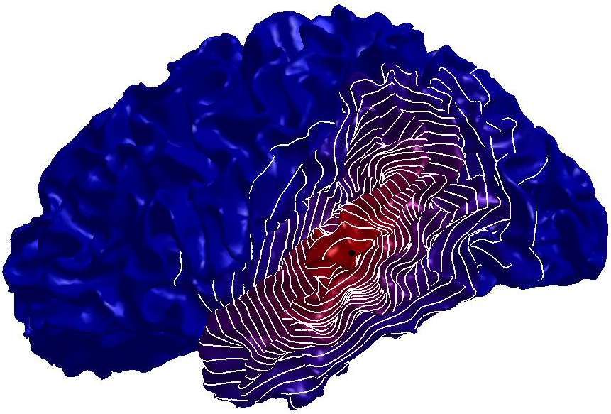
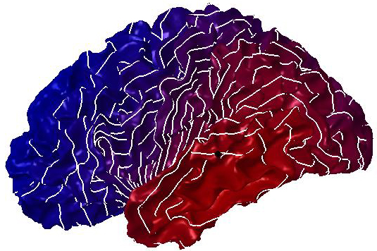
smoothness (Fig. 1a).
In previous work, the evaluation of the
L-curve is computationally expensive, as it generally involves the evaluation
of the Laplacian spectrum and/or the solution of a linear system with slowly
converging iterative solvers. Through the Padé-Chebyshev approximation,
we have an efficient way to evaluate the map ε(⋅) for
several values of t, thus precisely estimating the optimal time parameter. In
fact, the terms in Eq. (7) are evaluated by applying the Padé-Chebyshev
approximation of  and computing
  and
and  . In this way, we avoid the evaluation of the spectral
representations (7) through the computation of the Laplacian spectrum.
We consider the solution  to the heat diffusion process, whose initial condition takes value
1 at the anchor point
  and 0 otherwise. For our tests on triangle meshes, we have selected
the linear FEM weights [21, 26]. In this case [15], the discretization of the
  inner product is induced by the matrix B, which is intrinsic to the
surface
  and is adapted to the local sampling through the variation of the
triangles’ or Voronoi areas. In the paper examples, the level-sets are
associated to iso-values uniformly sampled in the range of the solution to the
heat equation, whose minimum and maximum are depicted in blue and red,
respectively. Furthermore, the color coding represents the same scale of values
for multiple shapes. Noisy examples have been achieved by adding a 20% Gaussian
noise to the input shapes.
Figure
6: Robustness of the
Padé-Chebyshev approximation with respect to surface sampling.
Truncated spectral and
Padé-Chebyshev approximations For the truncated spectral approximation  of the solution to the heat equation, the number k of eigenpairs
must be selected by the user and the approximation accuracy cannot be estimated
without extracting the whole spectrum. The different accuracy (Fig. 1b) of the
truncated spectral approximation and the Padé-Chebyshev method of the
heat kernel is analyzed by measuring the ℓ∞ approximation
error (y-axis) between the spectral representation of the heat kernel
  , computed using a different number k (x-axis) of eigenfunctions,
and the corresponding Padé-Chebyshev approximation. For small values of
t, the partial spectral representation requires a large number k of Laplacian
eigenvectors to recover local details. For instance, selecting 1K eigenpairs
the approximation error remains higher than 10−2; in fact, local shape
features encoded by
  are recovered for a small t using the eigenvectors associated with
high frequencies, thus requiring the computation of a large part of the
Laplacian spectrum. For large values of t, increasing k strongly reduces the
approximation error until it becomes almost constant and close to zero. In this
case, the behavior of the heat kernel is mainly influenced by the Laplacian
eigenvectors related to the eigenvalues of smaller magnitude. Indeed, the
spectral representation generally requires a high number of eigenpairs without
achieving an accuracy of the same order of the spectrum-free approximation
through the Padé-Chebyshev method.


Figure
7: Comparison of the accuracy of different
approximations of the heat kernel on the unitary sphere. ℓ∞ error (y-axis) between the ground-truth diffusion smoothing on the
cylinder, with a different sampling (x-axis) and scales. For different scales,
the accuracy of the Padé-Chebyshev method (r=5, orange line)
remains almost unchanged and higher than the truncated approximation
with 100 and 200 eigenpairs (red, blue line), the Euler backward
(green line) and power (black line) methods.
Table 1: Timings (in seconds) for the evaluation of
the heat kernel on 3D shapes with n points, approximated with k=500
eigenpairs (Eigs) and the Padé-Chebyshev approximation (Cheb.).
Column ’×’ indicates the number of times the computational cost is
reduced. Tests have been performed on a 2.7 GHz Intel Core i7 Processor,
with 8 GB memory.
|
Teeth Surf. (Fig. 3)
|
Brain (Fig. 5)
|
|
n
|
Eigs
|
Cheb.
|
×
|
n
|
Eigs
|
Cheb.
|
×
|
|
10K
|
39.01
|
0.32
|
122
|
20K
|
99.77
|
0.61
|
164
|
|
50K
|
154.13
|
2.50
|
62
|
50K
|
189.02
|
2.08
|
91
|
|
80K
|
188.21
|
4.12
|
46
|
100K
|
299.20
|
4.98
|
60
|
|
100K
|
307.03
|
6.21
|
49
|
200K
|
658.11
|
11.20
|
59
|
|
200K
|
450.21
|
10.03
|
45
|
400K
|
850.11
|
18.21
|
47
|
|
500K
|
670.31
|
21.11
|
32
|
500K
|
1001.11
|
32.11
|
78
|
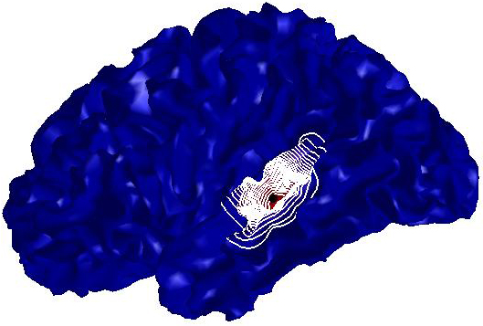
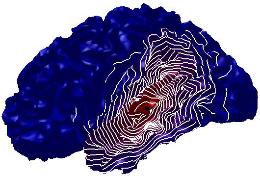
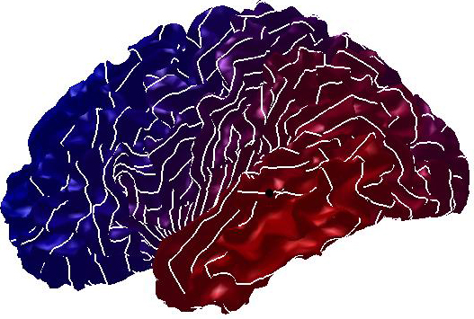
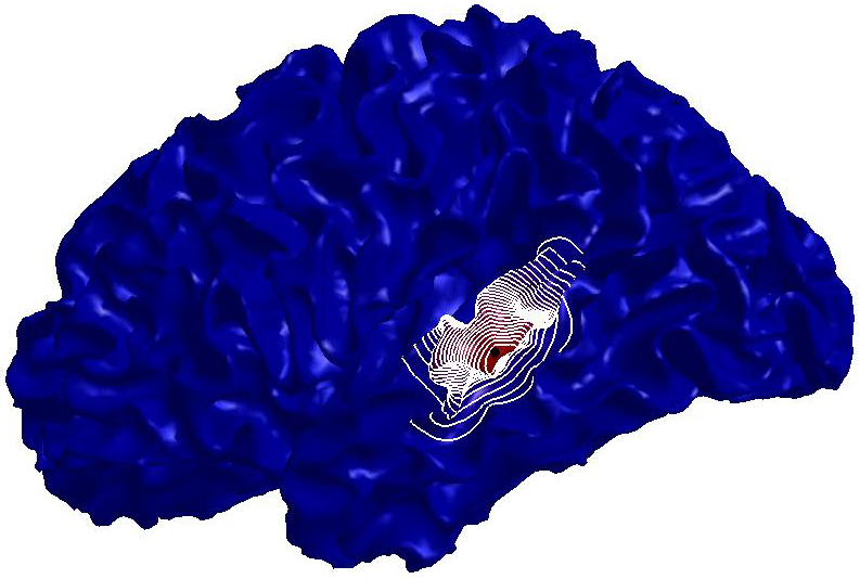
Robustness to noise and sampling. Figs. 2, 3, and 4 compare the diffusion smoothing of a noisy data
set computed with the Padé-Chebyshev approximation of degree r=7 and the
truncated approximation with k Laplacian eigenparis. A low number of eigenpairs
does not preserve shape details; increasing k reconstructs the surface noise.
For both examples, the ℓ∞ error
between (a) and the smooth approximation of (b) is lower than 1% for (c) the
Padé-Chebyshev method and (d) varies from 12% (k=100) up to 13% (k=1K)
for the truncated spectral approximation.
On irregularly-sampled and noisy shapes
(Figs. 5, 6), the spectrum-free computation provides smooth level sets, which
are well-distributed around the anchor point  and remain almost unchanged and coherent with respect to the
original shape. A higher resolution of
  improves the quality of the level-sets of the canonical basis
function, which are always uniformly distributed around the anchor (black dot).
Finally, an increase of the noise magnitude does not affect the shape and
distribution of the level sets.
We also compare the accuracy of the heat
kernel on the unitary sphere and computed with (i) the proposed approach; (ii)
the spectral representation of the heat kernel  , with k eigenpairs; (iii) the Euler backward method; and (iv) the
power method (Sect. 2). For all the scales (Fig. 7), the approximation accuracy
of the Padé-Chebyshev method is higher than the truncated Laplacian
spectrum with k eigenpairs, k=1,…,103, the Euler backward method, and
the power method. Reducing the scale, the accuracy of the Padé-Chebyshev
remains almost unchanged while the other methods are affected by a larger
discrepancy and tend to have an analogous behavior (t=10−4). Finally, the
Euler backward method generally over-smooths the solution, which converges to a
constant map as k→+∞, and the selection of m with respect to the shape details is guided
by heuristic criteria.

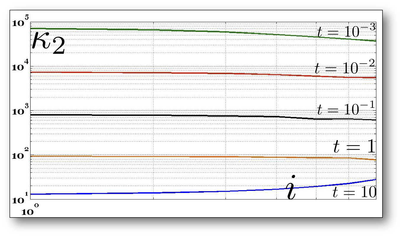
Figure
8: Numerical stability of the Padé-Chebyshev approximation. With
reference to Fig. 4, conditioning number κ2 (y-axis) of the matrices  , for different time parameters t; the indices of the coefficients
  are reported on the x-axis.
Numerical stability. According to Sect. 3, the scale t influences the conditioning
number of the coefficient matrices  , which are generally well-conditioned, as also confirmed by our
experiments (Fig. 8). While previous work requires to heuristically tune the
number of selected eigenpairs to the chosen scale, the Padé-Chebyshev
approximation has a higher approximation accuracy, which is independent of the
selected scale. Furthermore, those scales close to zero would require a larger
number of eigenpairs, thus resulting in a larger computational cost for the
truncated spectral approximation.
Computational cost. Approximating the exponential map with a (rational) polynomial of
degree r, the evaluation of the solution to the heat diffusion equation and the
evaluation of the heat kernel  at
at  is reduced to solve r sparse, symmetric, linear systems (c.f., Eq.
(5)), whose coefficient matrices have the same structure and sparsity of the
adjacency matrix of the input triangle mesh. Applying an iterative and sparse
linear solver (e.g., Gauss-Seidel method, conjugate gradient) [28] (Ch. 10),
the computational cost for the evaluation of the heat kernel and the diffusion
distance between two points is O(rτ(n)), where O(τ(n)) is the
computational cost of the selected solver. Here, the function τ(n), which
depends on the number n of shape samples and the sparsity of the coefficient
matrix, typically varies from τ(n)=n to τ(n)=n log n. In fact, O(n log
n) is the average computational cost of the aforementioned iterative solvers of
sparse linear systems. Timings (Table 1) are also reduced from 32 up to 164
times with respect to the approximation based on a fixed number of Laplacian
eigenpairs.
We have presented an efficient computation
of the diffusion soothing of medical data and the selection of the optimal
scale, which provides the best compromise between approximation accuracy and
smoothness of the solution. As future work, we foresee a specialization of the
spectrum-free computation and the selection of the optimal time parameter for
the analysis of brain structures and the smoothing of MRI images.
[1] L. Alvarez, P.-L. Lions, and
J.-M. Morel. Image selective smoothing and edge detection by nonlinear
diffusion. SIAM Journal on Numerical Analysis, 29(3):845–866, 1992.
[2] J.-M. Morel F. Catté,
P.-L. Lions and T. Coll. Image selective smoothing and edge detection by
nonlinear diffusion. SIAM Journal on Numerical Analysis, 29(1):182–193, 1992.
[3] P. Perona and J. Malik.
Scale-space and edge detection using anisotropic diffusion. IEEE Trans. on
Pattern Analysis and Machine Intelligence, 12(7):629–639, 1990.
[4] A. Spira, R. Kimmel, and N.
Sochen. A short-time beltrami kernel for smoothing images and manifolds. Trans.
on Image Processing, 16(6):1628–1636, 2007.
[5] T. Tasdizen, R. Whitaker, P.
Burchard, and S. Osher. Geometric surface smoothing via anisotropic diffusion
of normals. In Proc. of the Conference on Visualization, pages 125–132, 2002.
[6] A. P. Witkin. Scale-space
filtering. In Proc. of the Intern. Joint Conference on Artificial Intelligence,
pages 1019–1022, 1983.
[7] C. L. Bajaj and G. Xu.
Anisotropic diffusion of subdivision surfaces and functions on surfaces. ACM
Trans. on Graphics, 22:4–32, 2002.
[8] I. Guskov, W. Sweldens, and P.
Schröder. Multiresolution signal processing for meshes. ACM Siggraph,
pages 325–334, 1999.
[9] M. K. Chung, S. M. Robbins, F.
K. M. Dalton, C. R. J. Davidson, A. L. Alex, and A. C. Evans. Cortical
thickness analysis in autism with heat kernel smoothing. NeuroImage,
25:1256–1265, 2005.
[10] G. Wang, X. Zhang, Q. Su, J.
Chen, L. Wang, Y Ma, Q. Liu, L. Xu, J. Shi, and Y. Wang. A heat kernel based
cortical thickness estimation algorithm. In MBIA, volume 8159 of Lecture Notes
in Computer Science, pages 233–245, 2013.
[11] R. M. Rustamov. Multiscale
biharmonic kernels. Computer Graphics Forum, 30(5):1521–1531, 2011.
[12] R. M. Rustamov. Interpolated
eigenfunctions for volumetric shape processing. The Visual Computer,
27(11):951–961, 2011.
[13] A. Vaxman, M. Ben-Chen, and C.
Gotsman. A multi-resolution approach to heat kernels on discrete surfaces. ACM
Trans. on Graphics, 29(4):1–10, 2010.
[14] S. Lafon, Y. Keller, and R. R.
Coifman. Data fusion and multicue data matching by diffusion maps. IEEE Trans.
on Pattern Analysis Machine Intelligence, 28(11):1784–1797, 2006.
[15] G. Patanè. wFEM heat kernel:
Discretization and applications to shape analysis and retrieval. Computer Aided
Geometric Design, 30(3):276–295, 2013.
[16] L. Kobbelt, S. Campagna, J.
Vorsatz, and H.-P. Seidel. Interactive multi-resolution modeling on arbitrary
meshes. In ACM Siggraph, pages 105–114, 1998.
[17] U. Clarenz, U. Diewald, and M.
Rumpf. Anisotropic geometric diffusion in surface processing. In IEEE
Visualization, pages 397–405, 2000.
[18] M. Desbrun, M. Meyer, P.
Schröder, and A. H. Barr. Implicit fairing of irregular meshes using
diffusion and curvature flow. In ACM Siggraph, pages 317–324, 1999.
[19] F. Zhang and E. R. Hancock. Graph
spectral image smoothing using the heat kernel. Pattern Recognition,
41(11):3328 – 3342, 2008.
[20] G.G. Allaire. Numerical Analysis and
Optimization: An Introduction to Mathematical Modelling and Numerical
Simulation. Numerical Mathematics and Scientific Computation. Oxford University
Press, Incorporated, 2007.
[21] B. Vallet and B. Lévy.
Spectral geometry processing with manifold harmonics. Computer Graphics Forum,
27(2):251–260, 2008.
[22] D. K. Hammond, P. Vandergheynst,
and R. Gribonval. Wavelets on graphs via spectral graph theory. Applied and
Computational Harmonic Analysis, 30(2):129 – 150, 2011.
[23] M. Alexa and M. Wardetzky. Discrete
laplacians on general polygonal meshes. ACM Trans. on Graphics, 30(4), 2011.
[24] U. Pinkall and K. Polthier.
Computing discrete minimal surfaces and their conjugates. Experimental
Mathematics, 2(1):15–36, 1993.
[25] M. Belkin and P. Niyogi. Towards
a theoretical foundation for Laplacian-based manifold methods. Journal of
Computer System Sciences, 74(8):1289–1308, 2008.
[26] M. Reuter, F.-E. Wolter, and N.
Peinecke. Laplace-Beltrami spectra as Shape-DNA of surfaces and solids.
Computer-Aided Design, 38(4):342–366, 2006.
[27] A.J. Carpenter, A. Ruttan, and
R.S. Varga. Extended numerical computations on the 1/9 conjecture in rational
approximation theory. In Rational Approximation and Interpolation, volume 1105
of Lecture Notes in Mathematics, pages 383–411. Springer Berlin Heidelberg,
1984.
[28] G. Golub and G.F. VanLoan. Matrix
Computations. John Hopkins University Press, 2nd Edition, 1989.
[29] R.S. Varga. Scientific
computation on mathematical problems and conjectures. SIAM, CBMS-NSF regional
conference series in applied mathematics, 1990.
[30] P. C. Hansen and D. P. O’Leary.
The use of the l-curve in the regularization of discrete ill-posed problems.
SIAM Journal of Scientific Computing, 14(6):1487–1503, 1993.

