There are at least three different ways to
speed up a process of development of an numerical simulation application: choosing
the right architecture, using high level libraries and metaprogramming (code
generation), with help of computer algebra systems among other things.
Last decades shown that development on interpreted languages
which has dynamic typing (so called "duck typing", for example
Python, Ruby) is faster by an order of magnitude than development with aid of
traditional compiler-based languages with static typing (C/C++, Pascal,
Fortran). On the flip side, the resulting application
performance is low, Python application is 10-30 times slower than C++ one
depending on the problem type.
A numerical simulation program usually can be divided into
two parts the computational core and the interface. The computational core is
written with care. Its modifications are arguably rare since it has to provide
the best performance. Yet the interface is modified
continually to match different setups and its performance is of no importance since
the most part of computational costs fall on the computational core activities.
The ideal architecture for the numerical modelling
application is the combination of the interface written an interpreted language
with dynamic typing (we chose Python [1, 2]) and the computational core written
in an traditional compiler-based language which uses the static typing (aiwlib
is written in C++11). To connect the parts we are using SWIG tool [3]. The core
is compiled as the shared library and is imported to python as custom module.
This approach, for one, allows us to solve the calculation parameters assigning
problem efficiently. In the simplest case parameters values are listed in the
control file, which is written in Python, and they are edited on an as-needed
basis. The aiwlib library has its own build system based on GNU Make [4]. It
provides short (3-4 lines) user Makefile for such projects.
There are packages based on a similar architecture. A
well-known system Matlab uses its own interpreted language, which is focused on
implementing complex algorithms in terms of linear algebra, carrying out
calculation and visualizing the results. However, it is possible to implemented
an individual function in the C language and load it as shared library. The numpy library includes a number of algorithms applied mathematics
written in C and advanced visualization tools that are called from Python.
However, the Matlab system is commercial (with a fairly
expensive license). On top of that implementing an C extension to Matlab is not
an simple task. The numpy library is widely used (and in fact it is a
full-fledged replacement for Matlab), but the overhead for implementing complex
algorithms only in Python are too high, even if we take the calls of high-level
functions on C into account. Unlike analogues, the aiwlib
library instantiates main classes and function of the kernel written in C++11
to Python, which makes it possible to use almost the same code in both
languages, choosing the optimal decomposition of the application from the ratio
"code performance / development speed" point of view.
There is a persistent myth that numerical modeling applications
written in C++, are inferior in performance to applications written in Fortran.
In reality, it is much easier to write inefficient applications in C++ than in
Fortran, but obeying several simple rules [5], erase the difference in
performance. On the contrary, quite a few tools, provided to the developer in
modern C++ language, significantly speed up effective implementation of complex
computational algorithms. In particular, LRnLA (locally
recursive non-local-asynchronous) algorithms, which provide extremely high
performance in problems of numerical simulation [6, 7, 8, 9], were implemented
on combination of C++ and Python languages with heavy use of the C++ templates
mechanisms.
The choice of C++11 standard in aiwlib is
explained by the fact that, on the one hand, this standard gives a number new
features (for example, variadic templates), and on the other hand, it is
already well established and is supported by quite old compilers on most
current clusters and supercomputers.
The second way to accelerate the creation of a numerical
simulation applications is making use of high-level libraries. At the moment
there is a huge number of libraries that implement both complex data structures
(containers, for example, lists and various trees), and computational
algorithms (SLAU solvers, fast Fourier transform, etc.). Even if we limit
ourselves to C++ libraries we can mention boost, Eigen, gmm++ and MTL4 as
examples. The core of the aiwlib library is close to the library blitz++.
The aiwlib library complements the traditional functionality
of similar libraries with developed debugging tools, elements of linear algebra
with a number of specific operations, various containers (including arrays of
arbitrary dimension based on the Morton Z-curve and unique spherical grids
based on the subdivision of a dodecahedron), means of carrying out mass
calculations and developed means of visualization.
Visualization tools consist of the shell
for a standard gnuplot plotter, allowing with minimum effort to build a print
quality graphic, and a number of specific utilities for visualizing data on a
spherical grids, surfaces, distributions of magnetic moments, etc. Unlike
standard tools (eg paraview), aiwlib library viewers have a relatively poor window
interface (which is partly compensated by the developed command-line interface)
and are focused on handling large amounts of data.
The third way to accelerate the creation of numerical
simulation applications is the metaprogramming (automatic code generation) and
various systems computer algebra [10, 11]. There are some
tools in the aiwlib library for implementation of this approach (in particular,
converting algebraic expressions from Python language to gnuplot, C++ and LaTeX
formats is used in the gplt utility), but this is rather complex topic and is
beyond the scope of this article.
The previous version of the library aivlib (with the letter
"V", [12]) was successfully developed for over ten years, until it
became clear that the elimination of the accumulated list of drawbacks requires
breaking of the backward compatibility. This article is devoted to the second
version of the library which is referred to as aiwlib (with the letter
"W", [13]). Versions are incompatible but they can
be applied to one project simultaneously (from the point of view of the
compiler those are different libraries).
The aiwlib library provides advanced debugging tools which take
into account the specific nature of numerical simulation applications. The <aiwlib/debug> header file in C++ consists of
init_segfault_hook() function definition, the debug output macros WOUT and
WERR, the macro WCHK, checking the values of expressions for nan and inf, WEXT
and WEXC macros, which allow print information from the stack when an exception
is raised or a segmentation fault occurred, and WASSERT and WRAISE macros to
trigger an exception.
All macros print messages, which mention the source file,
line number and function, to the standard output stream or the standard error
stream. The macros (except the WRAISE macro) only work if the EBUG macro is
defined, for example, by using the "-DEBUG" compilation option or the
"debug=on" argument of make, otherwise, the macros are ignored by the
compiler. The macros listed can take as arguments an arbitrary number of
expressions. Here is the fragment of code
int a = 1; double b = 2.5; WOUT (a, a + b,
a * b + 3);
which after compiling and running will
print to the standard output stream the text
# test.cpp main () 14: a = 1, a + b = 3.5, a * b + 3 = 5.5
The WERR macro outputs information to the standard error
stream. It accepts any expression which result can be printed
to the stream std::ostream with the aid of the operator "<<".
The WCHK macro checks the values of its arguments (which
should be the results of evaluation of floating point number expressions) on
the values of inf and nan. If at least one argument did not
pass the check, an error message is displayed, and an exception is raised.
Macros WEXC and WEXT form special objects based on templates
std::tuple on the stack. Those objects contain copies of the arguments, that
practically does not affect the performance. When the stack frame is destroyed
(for example, the normal return from the function) objects with copies of macro
arguments are destroyed without side effects. When an uncaught exception is
raised or segmentation fault occurred the accumulated information is printed to
the standard error stream. The WEXC macro is thread ignorant thus it may be
used in multithreaded mode, but it does not handle segmentation faults. WEXT
macro works similarly, but it registers objects in the global table, hence it
is thread unsafe. If an segmentation fault occurs information from all the
objects registered in the global table is printed to the standard error stream.
To enable the processing of segmentation faults you must call
the function
init_segfault_hook();
This approach is often more convenient than a memory dump
analysis with the help of debugger. To begin with, the debugger can not show
the history of changes for arbitrary variable, while the WEXC and WEXT macros
can (this requires calling several macros). Secondly, when you
run your application on a supercomputer, the amount of memory to dump may
become too large for analysis.
When the processing of segmentation faults is enabled, a
call stack is also displayed. It can be analyzed by the standard addr2line
tool.
The first argument for the WASSERT macro should be a
condition. If its value is false, an exception is raised.
The aiwlib library provides I/O streams
(abstract base class aiw::IOstream and its successors aiw::File and
aiw::GzFile), based on the standard FILE streams and the zlib library. Aiwlib
streams differences from standard std::iostream streams are larger performance
(due to the elimination of an extra buffering), the availability a type-safe
analog of the printf method, the ability to map fragments of a file with automatic
garbage collection and operations "<" and ">", which
are overloaded as binary IO operations for all current data types and
containers, including STL types.
The aiwlib library defines the template for
the vector aiw::Vec<D, T=double>, parametrized by dimension (length) D
and cell type T (double is default). For this type traditional
operations addition, subtraction, scalar multiplication and comparison
operations (for an effective checking if the point lies in a D-dimensional
parallelepiped), componentwise multiplication, a module and maximum
calculations and so on are overloaded. The Vector type with int as the cell
type has an alias named aiw::Ind<D>. It is used as an index when
accessing cells of multidimensional grids.
A multidimensional area traversal operation
(D nested loops) is implemented:
aiw::Ind<D> N = ...; // size of an
area
for (Ind <D> i; i ^= N; ++ i) {...}
Typically, instantiating C++ templates to Python with SWIG
requires a special SWIG instruction for each instance of the instantiation. The
Instantiation is accompanied by the automatic generation and the compilation of
the large amount of C++ code, while the SWIG capabilities to handle C++11
standard extensions are limited. However, any alternative which allows binding
C++ and Python is significantly harder for an end user. Since the internal
representation of data in objects of the type Vec<D, T> is trivial, the
aiwlib library implements a special mechanism for instantiating such object,
based on the interaction with the SWIG type control system. Eventually for
vectors no instantiation is required: in Python it is enough to import a module
aiwlib.vec to get transparent access to objects Vec<D, T> (for all
current types T) which are present in the C++ code with all their capabilities.
In order to instantiate containers
described further (multidimensional and spherical grids) to Python, it is
necessary to assemble a separate module for each type and dimension using the
make utility, for example
make MeshF3-float-3
leads to the assembly of the module
aiwlib.MeshF3, containing a three-dimensional grid with float as the cells
type.
The most efficient approach for
implementing multidimensional arrays is to create in memory a traditional
one-dimensional array (vector) and emulate the multidimensionality with aid of
an address arithmetic. For this to happen it is necessary to define a
one-to-one correspondence between the index of the cell of the multidimensional
grid  and the offset in one-dimensional array f.
Obviously, there are many different
solutions to this problem, however the traditional way is the dictionary order
of cells

(1)
where the x-axis is the
"fastest", the data in memory is localized along the x-axis.
There are different axis orders available, for example, in
traditional multidimensional arrays of language C of the form T arr [Nx][Ny]...
the x axis is the "slowest". In general case, the traditional
solution can be written as

(2)
where  is the offset of the
zero cell,
  is the offset vector of the cell with the index (1,1,1 ...).
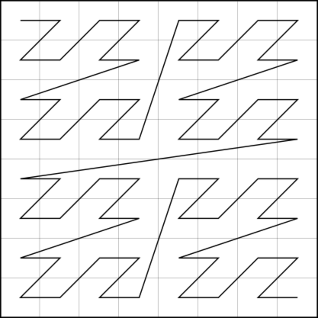
a.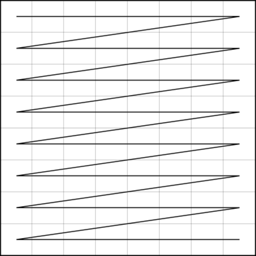 b.
b.
Fig. 1. Traditional
traversal of multidimensional array (a) and traversal based on Morton Z-curve
(b)
If a multidimensional array is a D-dimensional
hypercube with side size equals  cells the traditional approach
is reduced to constructing the offset f in the form

(3)
where k is the coordinate axis number (from
0 to D),  is the
  -th bit in
  . One can
suggest alternative order f

(4)
resulting in an order based on a fractal
Z-curve of Morton (Lebesgue) [14], Fig. 1.
In contrast to the traditional traversal,
one based on Z-curve significantly facilitates the construction of various
adaptive-recursive grids and ensures high locality of data (the nearest
neighbors in the configuration space, as a rule, are located close in memory). That
may increase the efficiency of calculations in the so-called memory-bound
problems [7, 8]. A fixed set of array sizes and low random access efficiency
are drawbacks of the Z-curve traversal. The calculation of the offset f by the
multivariate index of cell I is an fairly expensive operation from the
computational cost point of view.
The aiwlib library provides two array
classes Mesh<T, D> and ZCube<T, D>, parameterized by the type of
the cell T and the number of dimensions D of the array. The Mesh class
implements the traditional traversal and ZCube implements traversal based on
the Z-curve. Both classes have random access operator by multidimensional cell
index (an object of the type aiw::Vec<D, int>); efficient traversal for
the array and efficient access to the nearest neighbors of the cell, including
the periodic boundary conditions option; adjustment of uniform grids (limits
and step) and logarithmic scale on some axes, allowing to calculate the
coordinates of cell centers and cell corners in configuration space;
piecewise-constant, linear, local cubic and B-spline interpolation (can be
adjusted independently for individual axes); transposition (change of order)
and flip for axes; efficient saving data to disk and loading data from the disk
in binary and text formats in order to analyse or to visualize it later.
In addition, the Mesh class also allows you
to cut rectangular subdomains (grids of the same type, but smaller) and build
slices (meshes with less number of dimensions). Any grid conversion
(transposing, axis flipping or subdomain and slice cutting) returns a new grid
object which provides alternative access to the same data area. The memory allocation
and move operations for large amounts of data are not performed. In addition to
increase of the performance, that introduces extra opportunities for data
processing, for example, a two-dimensional section of a three-dimensional grid
may be filled with new data, which will lead to a change of the original
three-dimensional grid.
Furthermore, if necessary, it is possible
(by connecting the appropriate header file meshop) to overload the "unary
minus" operator, binary +, -, *, /, ^ (like in degree) operators and functions
abs, acos, asin, atan, ceil, cos, exp, fabs, floor, log, log10, sin, sinh,
sqrt, tan, tanh, atan2, fmod, pow over instances of Mesh <T, D> classes.
Expressions of arbitrary complexity are
allowed, so they may contain overloaded operations and functions whose operands
are instances of Mesh<T, D> classes or any other data for which the
expression will make sense if the instances of classes Mesh<T, D> are
substituted with values from one cell (type T).
The expression itself does not lead to any
action unless the operator "<<==" occurred, the left operand of
which must be an instance of the class Mesh<T, D> and the right is the
expression. In this case, a cycle is started on grid cells, on the left
hand side of the operation "<<==", for each grid cell on the
left the result of the expression on right hand side is calculated and is
written separately. The implementation is close to the grid-operator approach,
developed, for example, in [15].
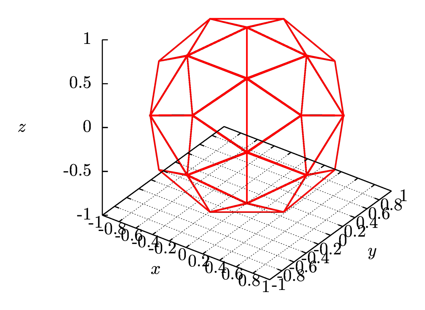
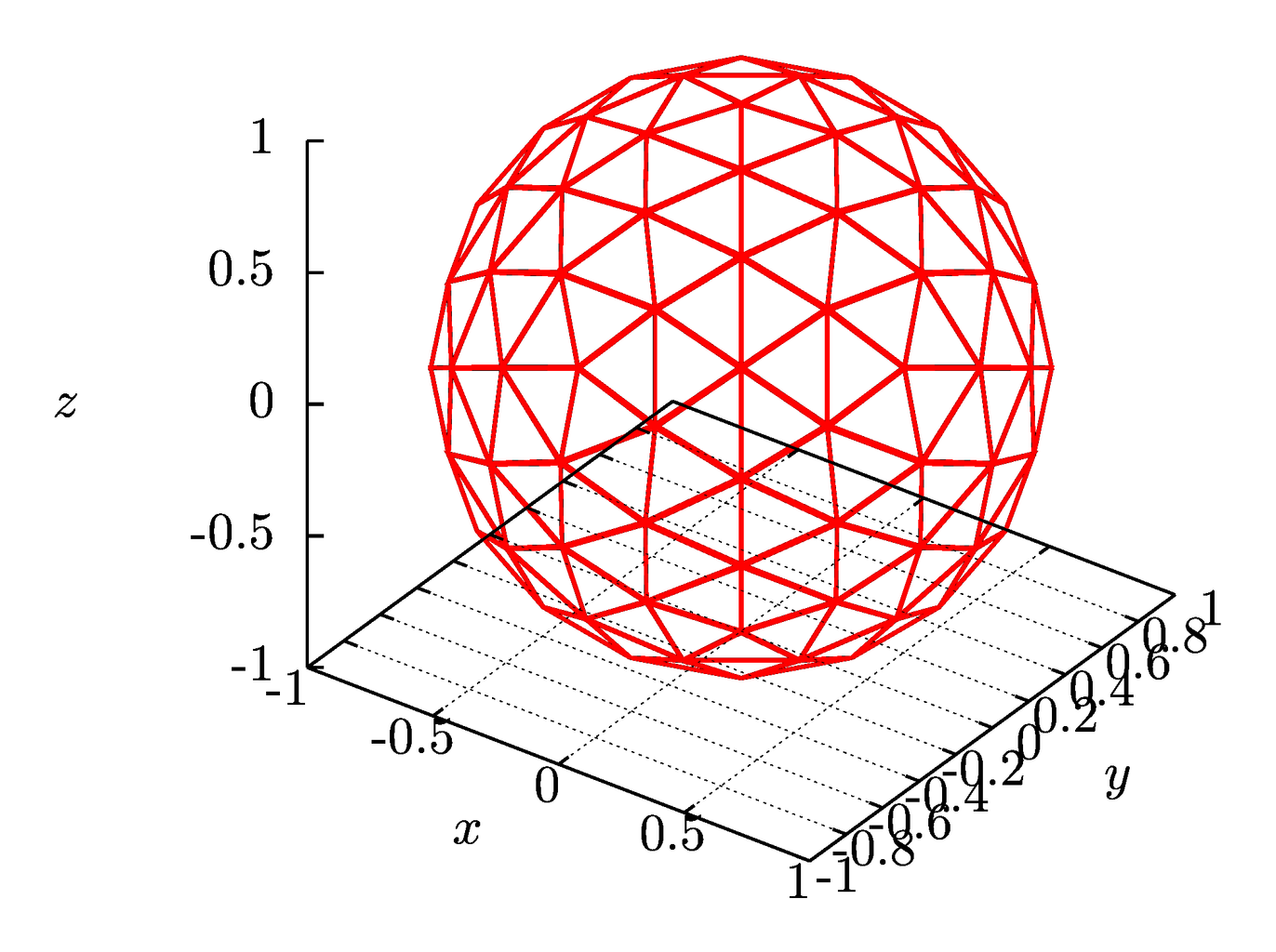
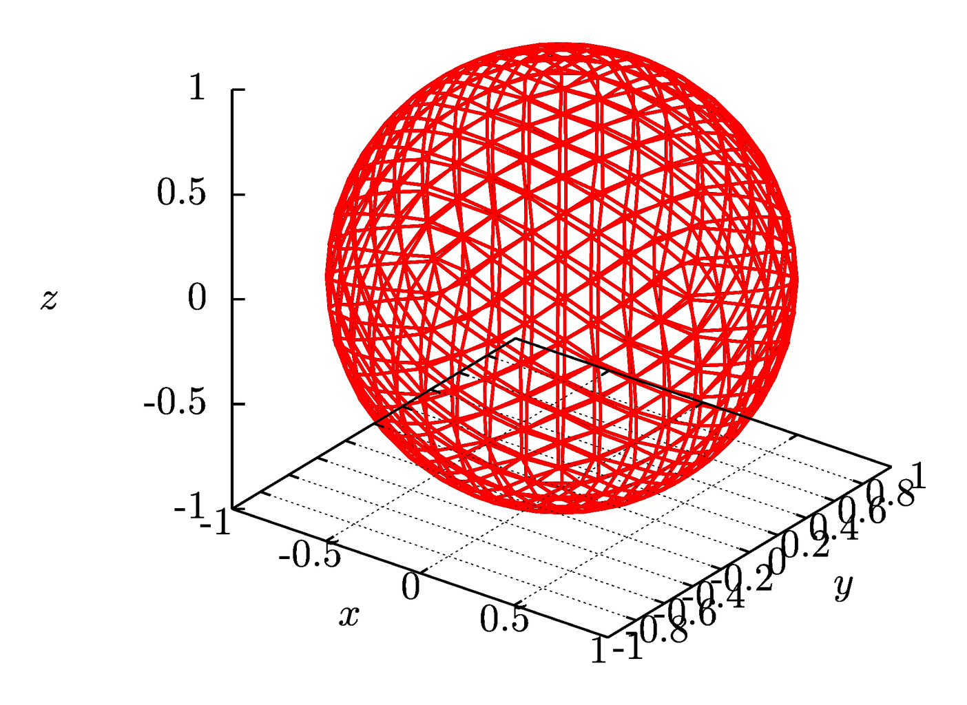
Fig.
2 Spherical mesh based on the recursive subdivisions of the dodecahedron with
different numbers of division steps (ranks).
The aiwlib library provides a mesh on a
sphere composed of almost regular triangles constructed by recursive
decomposition of the dodecahedron [16, 17], Fig. 2. Compared to
traditional spherical coordinates with two strong singularities on poles, a
spherical mesh based on a dodecahedron has 12 weak inhomogeneities
corresponding to centers of the dodecahedra faces. At these points the mesh
nodes are incidental to five cells, in contrast to six for all the remaining
nodes, and these cells are also most distorted (one of the angles is 72°
instead of 60°).
The mesh contains 60*4^R cells and 30*4^R+2
nodes, where R≥0 is the rank of the partition. A search for the
cell into which a three-dimensional vector points algorithm, the operations for
traversing the mesh and accessing to the neighbors of the cell, the algorithms
for calculation the coordinates of vertices, centers and areas for cells are
efficiently implemented.
The mesh is provided as the Sphere<T>
template, parameterized by a cell type, The template also includes methods for
writing and reading data in a binary format. In addition, there is an
utility for visualizing such data in the library. In numerical simulation a
spherical mesh is usually a convenient substitute for traditional spherical
coordinates, apart from the absence of strong singularities, a spherical mesh
with the same fineness (maximum cell size) requires approximately half the
number of cells due to absence of condensation of nodes near the poles.
Data from a spherical mesh can be saved to
and loaded from a disk in a binary format, and can also be visualized using the
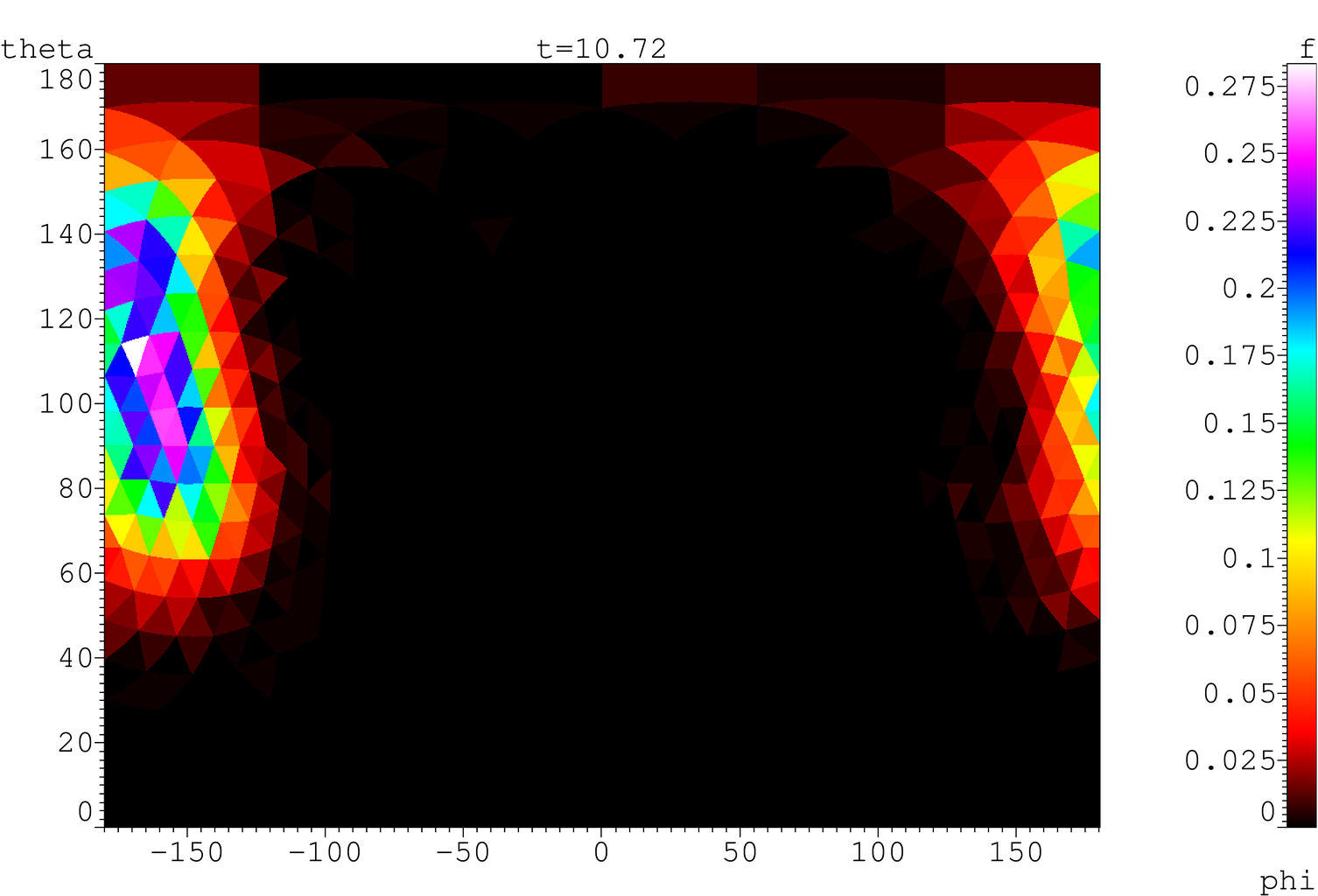
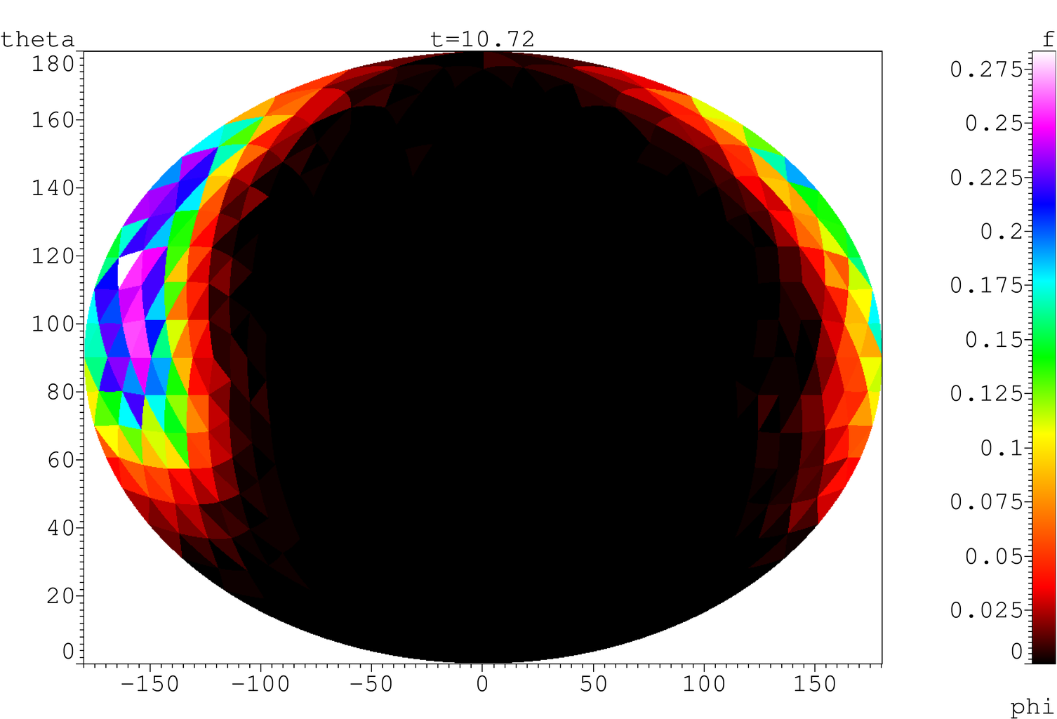
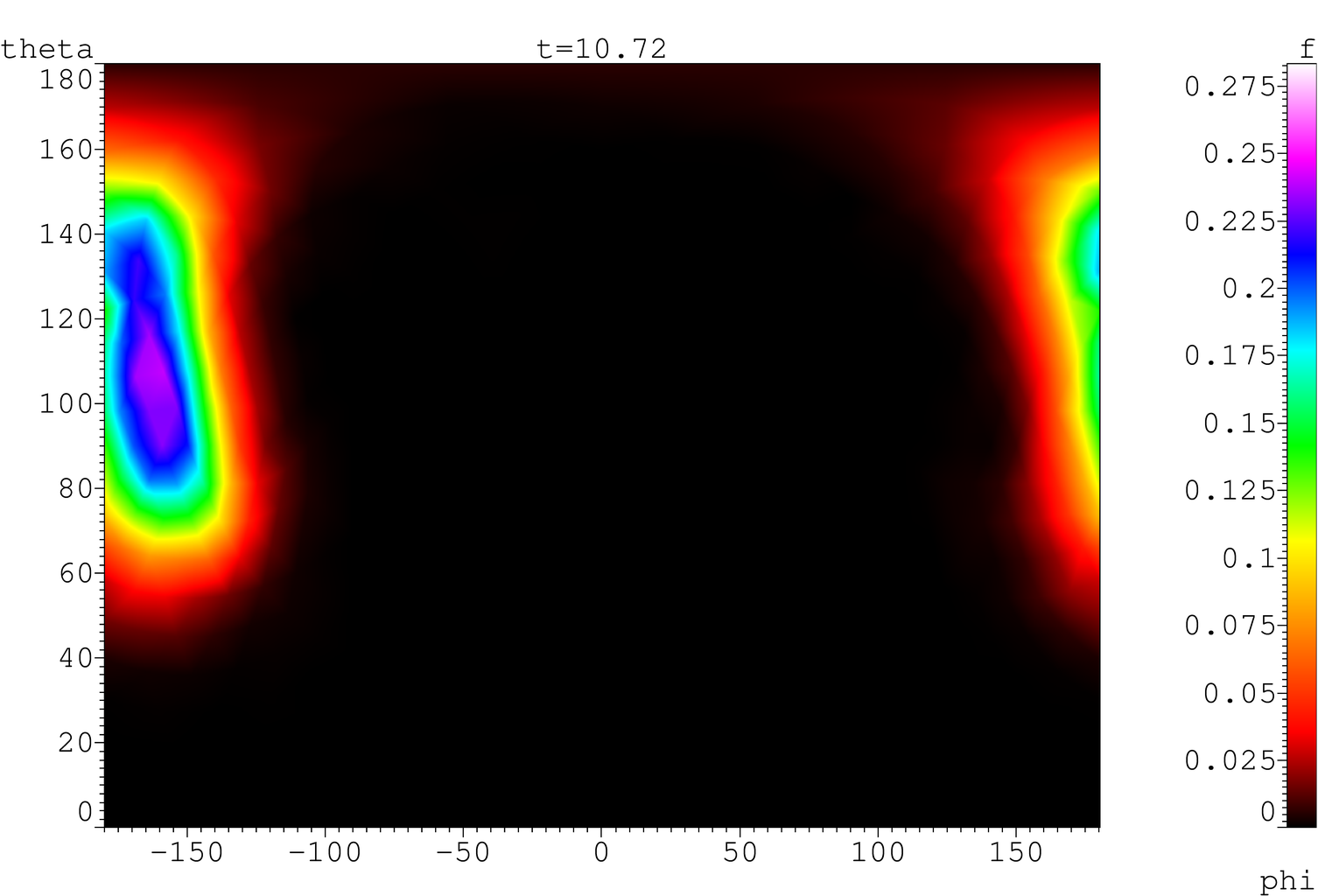
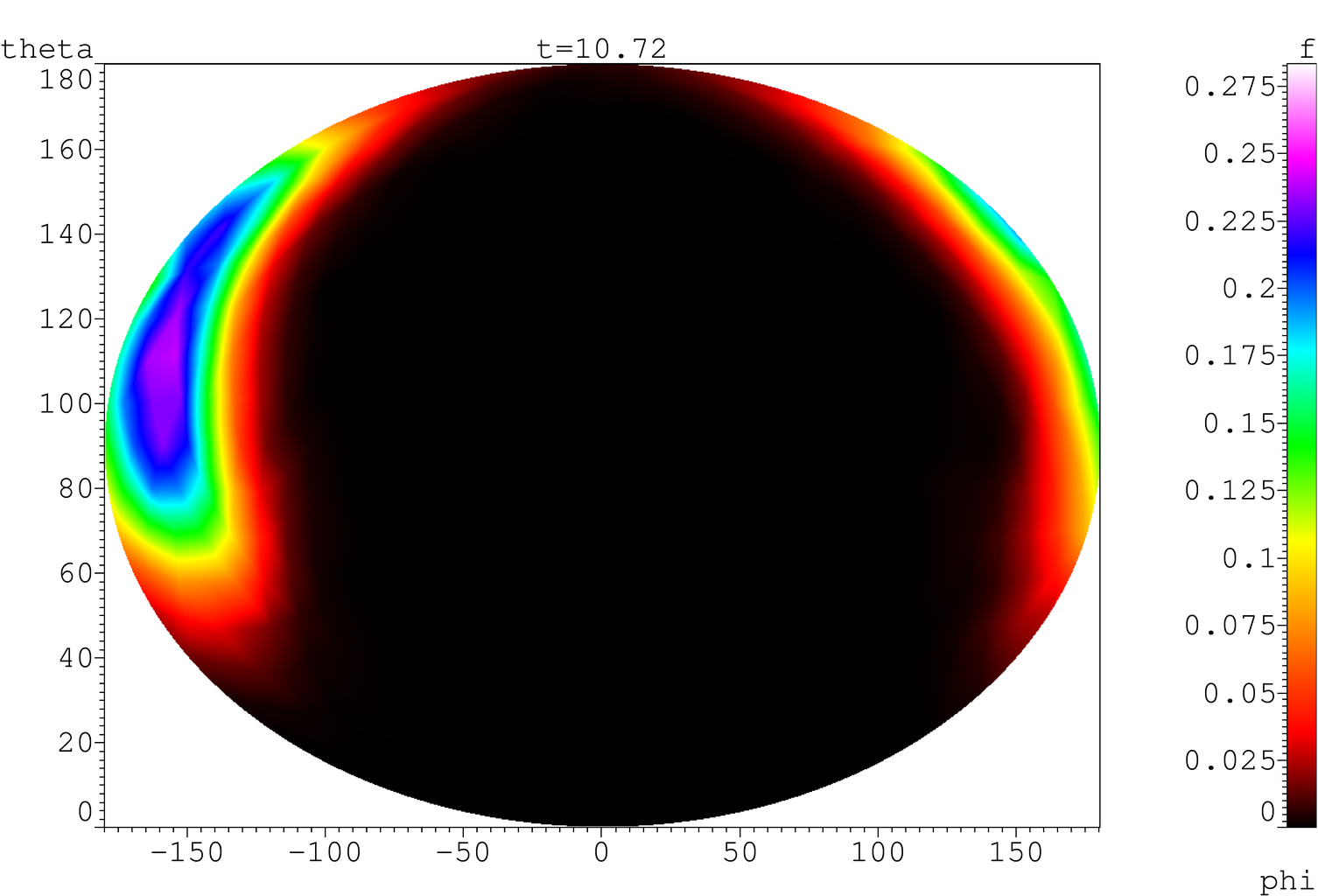
uplt viewer described below, Fig. 3.
Fig. 3. Visualization
of the distribution function of magnetic moments on a spherical mesh of the
third rank in the coordinates θ,φ without interpolation (a, b) and
with linear interpolation in cells (c, d) with aid of Mercator projection (a,
c) and with aid of Mollweide projection (b, d)
While performing numerical simulation, the
results of each calculation should be saved with the information on the
calculation parameters used and algorithms. Otherwise, the results tend
to turn into an abstract picture after a while. If there are quite a number of
methods and libraries to store parameters, yet saving of an algorithm is a
problem, and the only acceptable solution for it today is to store the source
code of the application as well.
When performing batch calculations (for
example, in the analysis of the behavioral dependence of a device on several
parameters and the calculation of its phase diagrams) requires a mechanism, which
allows us to start the application multiple times with different parameters
automatically. It also preferable to have control over the allocation of
resources within the framework of local network or a cluster.
To analyze the results, a multiparametric
search through the calculations is required. Thus the results of
calculations should be kept in special, ordered way. It should be possible to
search for specific versions of the source code. This problem may be solved
manually, for example, placing the results of calculations on a well structured
directory tree, but this approach requires a strict self-discipling of a user
and is tangled by the fact that during the calculation the order criteria may
expand and change dramatically.
For large series of calculations, a neat
solution to the above problems may take considerable amount of time and effort.
Several working groups have developed their own libraries, providing the
means to simplify the process of writing the environment [18, 19, 20], but
there is no unified approach for the problems.
The RACS system described in this section
(Results & Algorithms Control System, the system to control results and
algorithms) provides:
- setting the calculation parameters at startup
for applications written in Python and C++;
- automatic saving parameters and source codes for
each calculation;
- batch execution of calculations (cycled by
parameter values) and load balancing both on local machines and on clusters
with MPI;
- control points manipulation for C++
applications, even on clusters with MPI;
- advanced tools for multi-parametric searches,
analysis and results processing.
The following points were in focus while
the RACS was developed:
- easy usage (minimal modification of the debugged
code is required);
- concise and intuitive syntax when starting
calculations;
- the ability to process results using the
operating system and third-party utilities without losing the data integrity;
- Integration with other utilities, printing the
data in gnuplot format with gplt headers, reading metainformation about
calculations by other utilities.
Even for a low-skilled user, RACS
automatically provides necessary "minimum" of the calculation
self-discipline (storing of source codes and parameters). As a result, the user
is able to fully concentrate on dealing with his problem.
While developing the RACS system, special
effort was taken to facilitate the application of RACS on the finished program.
RACS is written in Python and is primarily aimed on applications, written
in C++ (high-performance computing core) and Python (upper control layer of the
application and the interface parts) linked together by the SWIG utility [3]. In
order to start calculations, RACS can be attached to applications written only
in C++ without using Python.
As a rule, the calculation starts from the
current (working) directory containing the source codes of an application, main
executables in Python or C++, etc. For each calculation in repository
(some directory) an unique directory is created. Calculation parameters, source
codes and simulation results are stored there. The set of calculation
parameters in form of a dictionary is saved as a file .RACS located in the
calculation directory. The format of .RACS is defined by the standard Python
module named pickle.
In addition to the .RACS file .src.tgz file
may be created in the unique calculation directory (archive containing the
source code of the application which performed the calculation) and in case of
"daemonized" calculation the logfile (standard output and standard
error streams combined) is also placed there.
The repository can be structured in an
arbitrary manner, i.e. it is the directory tree where calculations are grouped
according to user requirements (for example, by values of key parameters).
Individual calculations and repositories
can be moved by OS tools, sent over the network, etc.
The application is started as command line
instruction, but loading the RACS system adds extra command-line arguments
which make it possible to change the calculation parameters, to start batches
and to change the service parameters of the RACS system. It is possible
to start calculations batch looping through the list of the parameters values
and to balance the computer load induced automatically.
In order to analyze the simulation results
the racs command-line tool is introduced. There were attempts to create
a version with a GUI in 2010. However, it quickly became clear that the GUI
does not provide any advantages, but it complicates the interaction with other
command-line utilities essentially. It also introduce problems with remote work
through ssh.
The tool allows you to display the
dictionary of parameters for a separate calculation (contents of .RACS file),
to select the calculations that meet different criteria, to print selected
results in various formats, to modify selected calculations, or to delete them.
In fact, calculations placed under RACS
form a non-relational database, where individual calculations are the records
in the database, and repositories are the tables.
The racs tool is able to jointly process
multiple repositories. Repositories are processed sequentially (in the
order in which they were mentioned). Results are mergeed into a common
selection (set of calculations).
The racs tool gives the user broad opportunities for
multiparametric searching, analysing, joint processing and visualizing the
large volumes of numerical simulation results. To date (the first versions
appeared in 2003, the first publication [21] in 2007), RACS has proven itself
useful to organize large series of calculations in various fields, i.e.
seismic, modeling of the field development for kerogen-containing reservoirs with
in-situ combustion taken into account, modeling of magnetic systems [22] and the
development of spintronics devices [23], gasdynamics of the combustion [24],
the study of resonant properties of nonlinear systems [25], etc.
The gnuplot application is one of the
oldest visualization tools attributed to GNU project. Despite a number
of shortcomings (primarily the low performance, especially for surface plots) gnuplot
is still popular due to the flexibility, a variety of output formats and good
graphs appearance. The plotting graph of typographic quality (with the correct
fonts, axes labels, etc.) requires quite a lot of work. The gplt tool parses
command-line arguments, generates a set of instructions, and runs gnuplot. Since
the fact that many necessary parameters are set by default, and due to the
concise syntax, a minimum of actions (keystrokes) is required to obtain a
typographic quality plot in .pdf format with LaTeX fonts and formulas. In addition gplt-file containing the arguments of the corresponding
call is formed for each plot. One can edit the file to change the plot
if it become necessary.
The gplt tool is written in Python. It
reads the comments in .dat files (text files with data to render). Special
Comments (starting with #:) allows you to specify names for data columns,
declare additional numerical constants, customize the column names displayed on
plots for different output formats. The gplt tool is capable of using wide
variety of expressions (Python code snippets) containing the column names for
plotting. The gplt utility can also use metainformation (contents of .RACS
files) about calculations in expressions while plotting graphs for calculations
controlled by RACS system. The expression may be converted through abstract
syntax tree in gnuplot, LaTeX, EPS, and other formats.

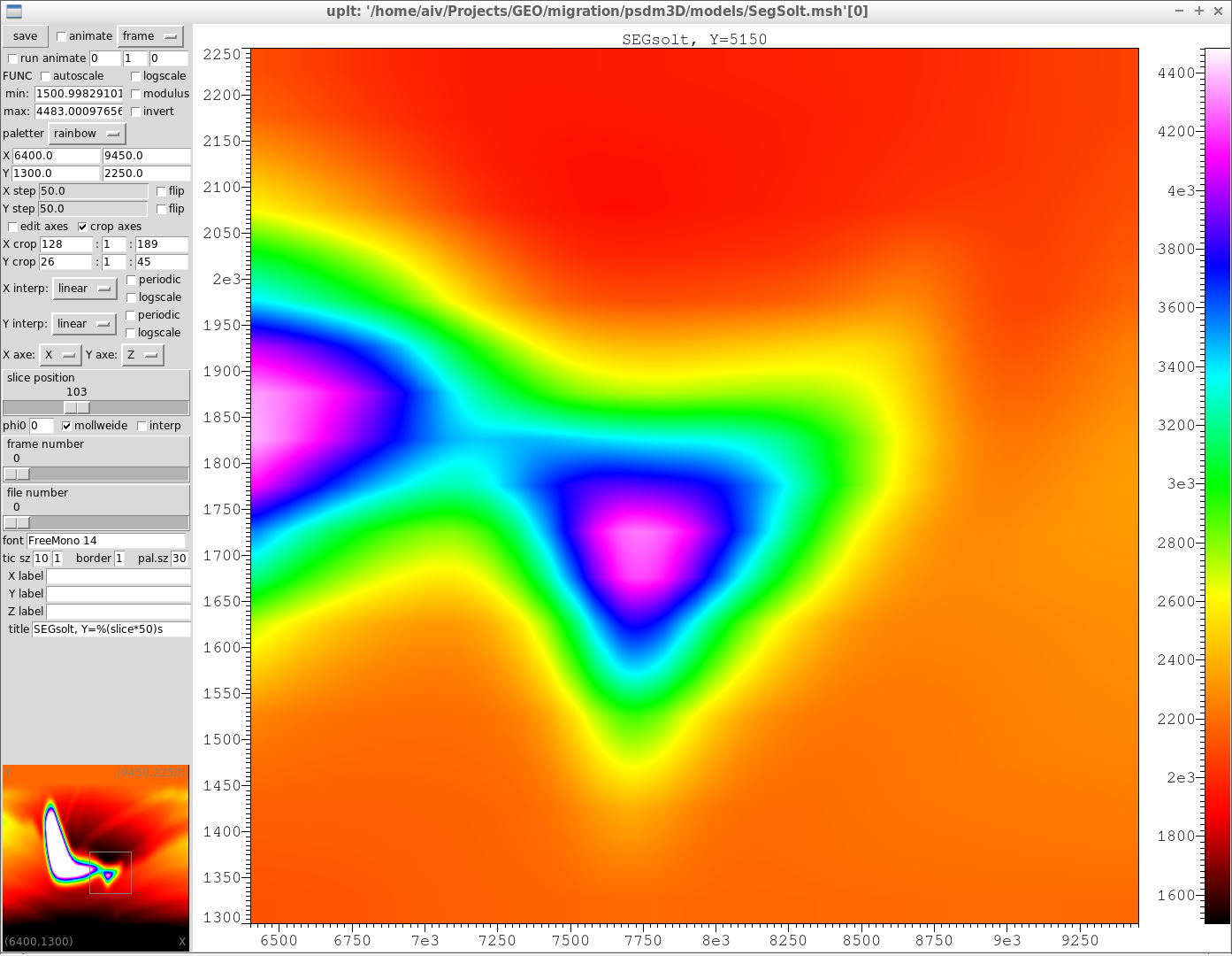
Fig. 4. Vertical
slice of the depth-velocity model for well known international synthetic
seismic dataset SEGsalt.
The uplt viewer is used to visualise the
scalar functions of the form f(x, y), defined on uniform rectangular meshes or
spherical meshes stored in the binary formats of the library aiwlib, Figure 4. The
viewer is implemented in C++11 and Python languages. It uses Tkinter library
and Python Image Library. In uplt viewer it is possible to adjust the palette
and limits of the image in many ways. Uplt also supports logarithmic scales for
any axis and different interpolation types. When the data written in one file
as the sequence of independent frames (each frame contains data from one mesh),
viewer allows you to navigate through the frames. For uniform meshes with
number of dimension greater than two, two-dimensional slices are displayed
instead of the full mesh. However the viewer makes it possible to select the
orientation and position of the cut. It is possible to start animation
(sequential drawing of files, frames in one file or movement of a slice through
one frame) and automatic video compiling with the ffmpeg utility.
Rendering options are set in two ways from
the graphical user interface and when the application starts with help of
command line arguments. Uplt also supports PDF as image output format.
Despite the fact that the viewer does not
utilise a graphics accelerator, viewer achieves acceptable drawing speed for
large (gigabytes or more) volumes of data.
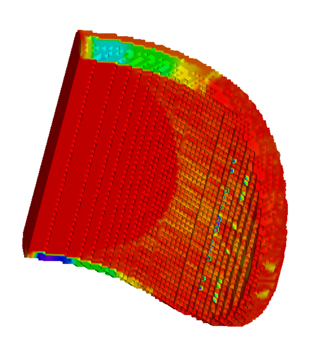
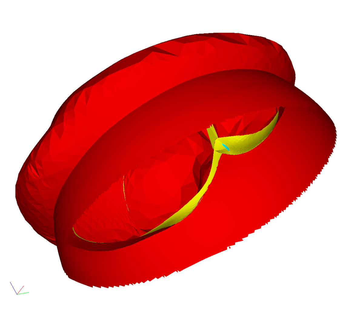
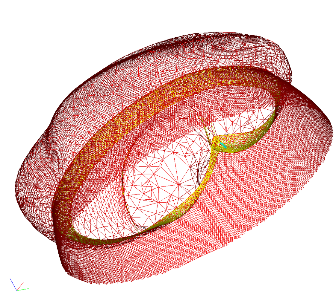
Fig. 5. Error level
on an unstructured tetrahedral grid during the evolution of a surface with a
movable boundary (a) and a wave front in the form of a surface during migration
on SEGsalt international seismic dataset (b) and a so-called "wire"
form for the same wave front (c)
The three viewers described below (splt,
mplt and fplt) are built with help of a separate package AbstractViewer, which
is not included in the aiwlib library. The package is focused on developing
new 3D viewers in C++ and Python languages using OpenGL library and glut. It
also permits to embed viewers in numerical simulation applications for
displaying and analysis results during the calculations on GPGPU. The package
was developed by S. Khilkov and is distributed under the GPL-v3 license.
Due to the efficient use of a discrete
video card, viewers have high performance. The interface is made in a
deliberately "Spartan" style, the manipulator "mouse"
allows you to rotate the image, all other actions are performed with aid of
hotkeys and command line interface in the terminal. The command line uses the
readline library, which provides autocomplete feature for the input buffer and
access to the commands history. Terminal commands are executed in Python
language, which makes it possible to to run scripts for generation a series of
images, creation of the animation, etc.
All viewers supports palettes switching and
color range limits adjustments. They implement clipping planes, scaling
and rotating transformations of the image.
The splt viewer can display quite an
arbitrary surface defined by an unstructured triangular grid (Figure 5), while
tetrahedral grids are specified as sets of faces. Grids are stored in a
binary format of aiwlib library. An arbitrary number of independent frames (instant
grid states) could be placed in a single file consecutively. Grids in different
frames may have different numbers of nodes and vertices. Viewer
implements an efficient switching between frames.
Arbitrary data sets of type float4 may be
associated with vertices and cells of a triangular grid (for example,
coordinates and components are associated with vertices speed, and density is
defined at cell centers). Each data field has an unique text name. During
the visualization, it is possible to select arbitrary combinations of fields, the
values of three fields are plotted along the axes xyz, the value of the fourth
field is shown as the color. It uncovers broad potential for visualization and
analysis of complex data, the detection of various dependencies and then
studying their evolution in results of calculations.
|

|

|
|
a
|
b
|
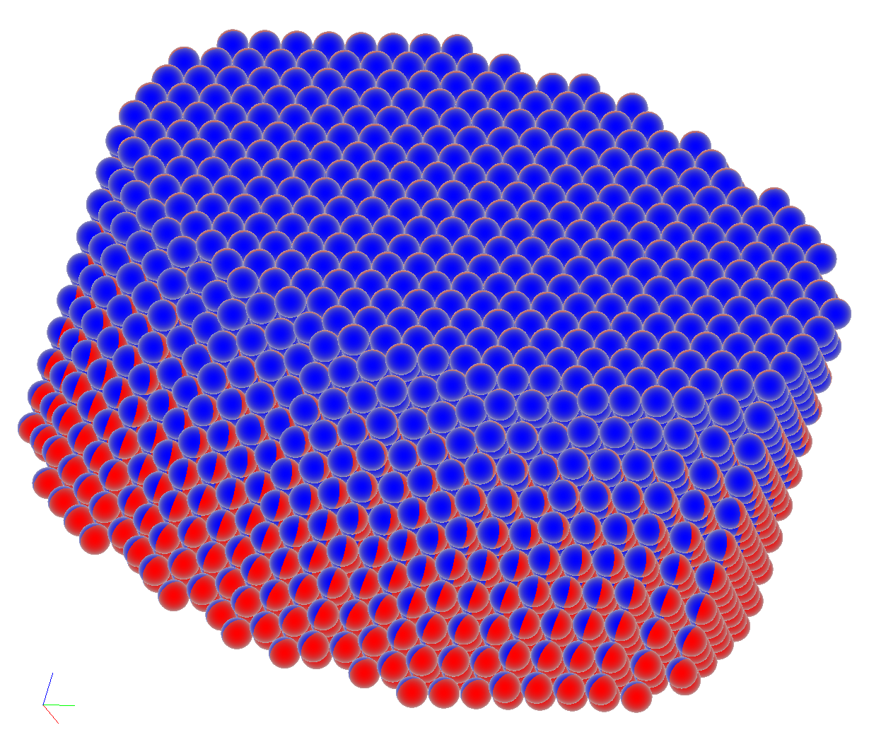
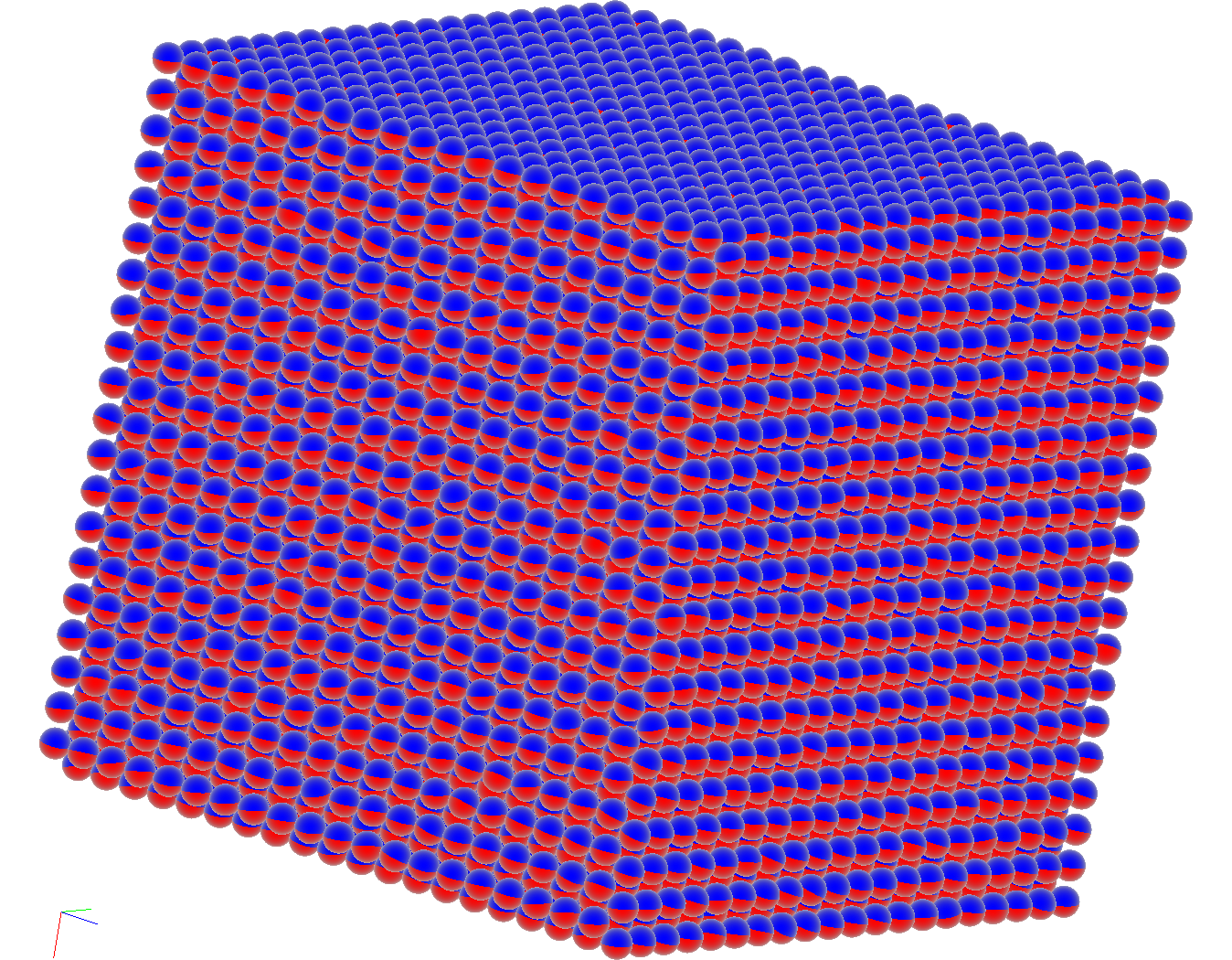
Fig. 6. Distribution
of magnetic moments in the cylinder made of antiferromagnetic material which
has incomplete fcc lattice (a) and for a cube made of ferromagnetic material
with bcc lattice (b)
In order to visualize the distribution of magnetic moments,
the aiwlib library provides the mplt viewer. The magnetization of a single
cell/atom is represented by red and blue sphere (similarly to compass arrow)
which blue pole is oriented along the magnetic moment direction. A
three-dimensional array of such spheres conveys the distribution magnetization
on the surface of the sample well (inner spheres are virtually not visible,
Fig. 6).In order to study the magnetization distribution within the sample it
is necessary to use slices and/or cut-off planes.
The viewer works with the data stored in a
special binary format of the aiwlib library. The simulation results are
stored in one file, which consists of a header describing the spatial
distribution of the magnetic moments and data frames after it. Each frame
contains the values of the magnetic moments at some point in time. To store the
orientation of a single magnetic moment one can use either a vector of three
float4 numbers (12 bytes), or the cell number on the spherical grid built with
help of a recursive decomposition of a dodecahedron of the rank five (2 bytes,
the accuracy is approximately 1°). The viewer efficiently displays arrays of up
to 10^9 magnetic moments, the only limit is the video memory size.

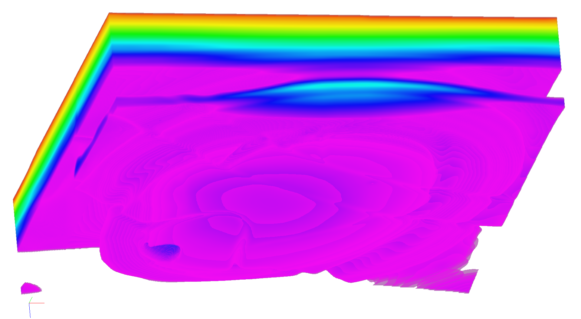
Fig.7. Three-dimensional image of a velocity-depth model of a known international
synthetic seismic dataset SEGsalt.
The fplt viewer provides the voxel
visualization of uniform 3D meshes saved in aiwlib library formats, figure 7. A
pixel shader traces rays with an increment of the order around the grid cell
size, taking transparency into account. The initial value (color) is considered
invisible (completely transparent), the tracing of each ray is completed after
achieving a given value in the pixel α-channel (default value is 0.95)
[26] or if the ray escapes the data area.
The aiwlib library has a number of
additional modules for solving various specific tasks.
The construction of isolines which is
implemented in C++; control points for stopping and continuing the calculation;
serialization of data in the pickle format; the discretization of a Voronoi
partition; means to collect and to store the metainformation about custom data
types (structures) to use in postprocessing of calculations results; some
elements of linear algebra and analytical geometry, including the projection
construction and rotation operations; means for reading/writing test
configuration files and configuring user objects.
An efficient way to parse the command-line
arguments, allowing you to create your DSL (Domain-Specific Languages)
implemented in Python; high-level module to work with date and time; the
automatic detection of files containing the source code of the application
written in C++ and Python languages, combined by the SWIG utility and compiled
with make; the cost effective protocol for transferring data through sockets
and high-level tools for developing simple network client-server applications;
the conversion algebraic expressions from the Python language format into other
formats with aid of the abstract syntax tree.
The first version of the aiwlib library was
written in 2008, and some of its parts (the RACS system and the gplt tool)
appeared in 2003. Over the years the library code evolved dramatically.
The kernel code became simpler, smaller, more stable, and its capabilities
significantly expanded.
The aiwlib library and its previous version
aivlib were used successfully in a number of projects: development software
packages for the seismic prospecting [27, 28, 29], the physics of plasma [6]
and the optics of turbid media [30]; solutions to fundamental and applied
problems in analysing of magnetic materials and thecreation of spintronics
devices [22, 23]; the research on resonance properties of superparamagnets
[25]; simulations of the gas dynamics and the combustion [24], processes of the
field development for kerogen-containing oil reservoirs, taking the in-situ
burning into account, the material degradation and the blistering in the
subsurface layers under the influence of the ion bombardment [31]; modeling of
problems of poroelasticity and hydraulic fracturing of the formation [32]. In
the meantime, the developed of visualization tools of the library played the
important role in those projects. Due to efficient analysis of simulation
results, debugging code and the adaptation of numerical schemes to the problems
in question were greatly simplified.
The core of the library is distributed
under the license Apache-2 (which permits to apply it in commercial projects
with a closed source code), and visualization utilities are distributed under
the GPL-3 license.
The aiwlib library development is
continuing actively. We are intended to include in the library modules for
the CUDA language, as well as templates (frameworks) for creating magnetic
materials simulation codes and various variants of FEM/XFEM, since we have
acquired sufficient experience in those areas.
[1] Guido van Rossum, and Fred L. Drake, Jr. Jazyk programmirovanija Python. Russian
translation by Denis S. Otkidach. [An Introduction to Python]. 2001. [In Russian]
[2] Mark Lutz. Programmirovanie na Python [Programming Python] (Second Edition). 2002 [In Russian]
[3] Simplified Wrapper and Interface Generator http://www.swig.org
[4] Richard M. Stallman, Roland McGrath. GNU Make: A Program
for Directed Compilation. Free Software Foundation 2010
[5] Scott Meyers. Effective Modern C++. O`REILLY. 2016.
[6] A. Yu. Perepelkina, I. A. Goryachev, V. D. Levchenko
CFHall Code Validation with 3D3V Weibel Instability Simulation. //Journal of
Physics: Conference Series. IOP Publishing. — 2013. — V. 441. — No. 1. — P.
012014
[7] A. Yu. Perepelkina, V. D. Levchenko, I. A. Goryachev
Implementation of the Kinetic Plasma Code with Locally Recursive non-Locally
Asynchronous Algorithms. // Journal of Physics: Conference Series. — IOP
Publishing. — 2014. — V. 510. — No. 1. — P. 012042
[8] V. D. Levchenko, A. Yu. Perepelkina, A. V. Zakirov.
DiamondTorre Algorithm for High-Performance Wave Modeling. // Computation 4.3
(2016): 29.
[9] V. D. Levchenko, A. Yu. Perepelkina. The DiamondTetris
Algorithm for Maximum Performance Vectorized Stencil Computation.
//International Conference on Parallel Computing Technologies. Springer, Cham.
— 2017. — P. 124–135.
[10] Tan Kiat Shi, Willi-Hans Steeb and Yorick Hardy “Symbolic C++: An
Introduction to Computer Algebra using Object-Oriented Programming”, 2nd
extended and revised edition. Springer. 2000
[11] S.A. Zhdanov, A.V. Ivanov. Primer avtomaticheskoj generacii koda prilozhenija chislennogo modelirovanija dlja reshenija uravnenija Fokkera–Planka [Example of automatic code generation of numerical modeling application for solution of the Fokker–Planck
equation]. // Matematicheskoe modelirovanie. — 2015. — V. 27. — No 9. — P. 49–64. [In Russian]
[12] A.V. Ivanov, Khilkov S.A., S.A. Zhdanov. The Aivlib
library. http://a-iv.ru/aivlib/
[13] A.V. Ivanov, Khilkov S.A. The Aiwlib library. https://github.com/aivn/aiwlib/blob/master/doc/aiwlib.pdf
[14] G. M. Morton. A computer Oriented Geodetic Data Base;
and a New Technique in File Sequencing. — Ottawa, Canada: IBM Ltd., 1966. —
(Technical Report).
[15] M.M. Krasnov. Metaprogrammirovanie shablonov C++ v zadachah matematicheskoj fiziki [Metaprogramming
C++ templates in mathematical physics problems]. - Moscow: Keldysh Institute
Applide Mathematics. - 2017. - 84 P. [In Russian]
[16] A.V. Ivanov. Kineticheskoe modelirovanie dinamiki magnetikov [Kinetic modeling of magnetic's dynamics].
// Matematicheskoe modelirovanie. — 2007. — V. 19. — No 10. — P. 89-104. [In Russian]
[17] S.A. Khilkov, A.V. Ivanov Numerical simulation of the
magnetic moment distribution evolution for superparamagnetic materials
//Preprints of Keldysh Institute Applide Mathematics. — 2014. — No 29. — P.
1-16.
[18] A.E. Alexandrov, A.V. Tyurin. Programmnye instrumental'nye sredstva dlja organizacii vychislitel'nogo jeksperimenta s cel'ju provedenija mnogovariantnogo analiza [Software tools for
computing experiment aimed at multivariate analysis implementation]. // Nauchno-tehnicheskij vestnik informacionnyh tehnologij, mehaniki i optiki [Scientific
and technical journal of information technologies, mechanics and optics]. -
2015. — V. 15. — No 5. — P. 907-915. [In Russian]
[19] Mnogovariantnyj analiz. Programmnyj kompleks dlja avtomatizacii modelirovanija nestacionarnyh processov v mehanicheskih sistemah i sistemah inoj fizicheskoj prirody [The software for simulation of non-stationary processes
in mechanical systems and systems of other physical nature].
http://www.laduga.ru/pradis/help/pradis/PRADIS_Multivaria_analysis.ru.htm [In Russian]
[20] B. M. Adams. at al. Dakota, A Multilevel Parallel
Object-Oriented Framework for Design Optimization, Parameter Estimation,
Uncertainty Quantification, and Sensitivity Analysis: Version 6.6 User’s
Manual. —SAND2014-4633. — 2017. — P. 1–319. https://dakota.sandia.gov/
[21] A.V. Ivanov. Sistema kontrolja rezul'tatov i algoritmov dlja zadach chislennogo modelirovanija [Results and algorithms control system for
digital modeling tasks]. // Automation. Modern
technologies. - 2007. - No 12. - P. 29-34. [In Russian]
[22] S.A. Khilkov, A.V. Ivanov, E.V. Zipunova. Numerical simulation of strongly nonequilibrium processes in magnets
based on physical kinetics equations // Mathematical Models and Computer
Simulations. — 2016. — V. 8. — No 6. — P. 703-708.
[23] I.M. Iskandarova, A.V. Ivanov, A.A. Knizhnik, A.F.
Popkov, B.V. Potapkin, K.A. Zvezdin, P.N. Skirdkov, Q. Stainer, L. Lombard, K.
Mackay. Simulation of switching maps for thermally assisted
mram nanodevices // Nanotechnologies in Russia. - 2016. - V. 11. - № 3-4. - P.
208-214.
[24] M.A. Liberman, M. Kuznetsov, A. Ivanov A., I. Matsukov.
Formation of the preheated zone ahead of a propagating flame
and the mechanism underlying the deflagration-to-detonation transition
//Physics Letters A. — 2009. — V. 373. — No 5. — P. 501-510.
[25] S.A. Khilkov, A.V. Ivanov Rezonansnye svojstva superparamagnetikov pri malyh amplitudah vneshnego periodicheskogo polja [Resonant properties
of superparamagnetic materials for small amplitudes of the periodic field]
// Matematicheskoe modelirovanie. — 2015. — V. 27. — No 8. — P. 96-110. [In Russian]
[26] CUDA Toolkit Documentation: Volume
Rendering with 3D Textures http://docs.nvidia.com/cuda/cuda-samples/index.html#volume-rendering-with-3d-textures
[27] V. D. Levchenko, A.Yu.
Perepyolkina, A.V. Ivanov, A.V. Zakirov, Т.V. Levchenko, V.E.Rock. Vysokoproizvoditel'noe dinamicheskoe 3d modelirovanie polnovolnovogo sejsmicheskogo polja v zadachah sejsmorazvedki. Opyt primenenija v uslovijah razlichnyh sejsmo-geologicheskih regionov [High-performance dynamic 3d modeling of full-wave seismic field in seismic survey problems. experience in various seismogeological regions] // Supercomputer
technologies in the oil and gas industry. Mathematical
methods, software and hardware Materials of scientific practical conference. -
2017. - P. 49-53. [In Russian]
[28] A.V. Zakirov, V.D. Levchenko, A.V. Ivanov, A.Yu. Perepelkina, Т.В. Levchenko, V.E. Rock Vysokoproizvoditel'noe 3d modelirovanie polnovolnovogo sejsmicheskogo polja dlja zadach sejsmorazvedki [High-performance 3d modeling of a full-wave seismic field for seismic prospecting] // Geoinformatics.
- 2017. - No. 3. - P. 34-45. [In Russian]
[29] A.L. Pleshkevich, A.V. Ivanov, V.D.
Levchenko, S.A. Khilkov. Mnogoluchevaja 3D glubinnaja sejsmicheskaja migracija do summirovanija s sohraneniem amplitud [Multibeam 3D depth seismic migration before summation
with preservation of amplitudes] // Geophysics. specialist.issue "50 years
of CGE". - 2017. - P. 89-97. [In Russian]
[30] A.V. Dmitriev, A.V. Ivanov, A.R.
Khokhlov Numerical simulation of light propagation through a diffuser // Journal
of Mathematical Sciences. — 2011. — V. 172. — No 6. — P. 782-787.
[31] G.I. Zmievskaya, A.L. Bondareva. Kinetics
of the formation of pores and a change in the properties of materials in
numerical model //Journal of Surface Investigation: X-Ray, Synchrotron and
Neutron Techniques. — 2016. — V. 10. — No 4. — P. 802-808.
[32] A.V. Ivanov, E.B. Savenkov. Modelirovanie i vizual'noe predstavlenie dinamiki poverhnosti s podvizhnym kraem na stacionarnoj nestrukturirovannoj setke [Simulation and
visualization of the dynamics of a surface with a movable boundary on a
stationary unstructured mesh]. //Scientific Visualization. - 2017. —V. 9. — No
2. — P. 64–81. [In Russian]

 b.
b.