The
visualization method presented herein was conceived within the context of
investigating nonlinear systems exhibiting deterministic chaotic dynamics
[1-3]. Two fundamentally divergent approaches to studying chaotic systems
exist; in a sense, both are philosophical constructs.. The
first, conventional approach employs the methods of classical continuum
mathematics. The second is predicated upon A.N. Kolmogorov's theory of
algorithmic information, known as Kolmogorov complexity [4], which is grounded
in the concept of finite precision. The conceptual framework of Kolmogorov
complexity constitutes the conceptual underpinning and primary motivation for
our research. Within Kolmogorov's framework, as applied to chaotic systems, the
classical conception of a trajectory is absent. Instead of trajectories — deemed
uncomputable by Kolmogorov — one must consider either solutions obtained
through regularization/discretization or functionals thereof. The computational
method (algorithm), serving as the sole instrument for "observing"
trajectories, becomes an integral component of the system itself. An analogy
with quantum mechanics is apt: the equations governing the system's evolution
assume the role of quantum objects, the act of observation consists in
introducing regularization — practically manifested in the application of a
specific numerical method — and the computational outcomes become the
observables.
The
implementation of any numerical method on a computational device inherently
entails the discretization of the mathematical object under study. It is obvious
that should the computation of a phase trajectory on a strange attractor be
prolonged sufficiently, the trajectory will eventually close upon itself, a
consequence of the finite precision and determinism of the computing machinery.
Thus, the "observed" strange attractors "materialize" as
sets of cycles. In [1, 2], systematic investigations into the
discrete analogues of strange attractors, wherein the discretization scheme was
specifically tailored to reflect the fundamental properties of algorithmic
computation were undertaken. We herein recapitulate several pivotal findings.
The
precision of discretization, formally expressed by the lattice step size in the
system's phase space, dictates the ultimate complexity of the cycles comprising
the discrete attractor. As the lattice step is refined, the complexity of these
cycles increases predictably, while the average number of cycles remains
largely conserved. The deliberate use of the term "ultimate
complexity" is warranted, as minor perturbations of the lattice step
around any given value yield not only discrete attractors of the maximum
permissible complexity but also variants of any lesser complexity. A veritable "spectrum"
of cycles emerges, representatives of which can be obtained with a certain
probability by varying the discretization parameter. It is a curious fact that
even under fine discretization — where the cycle set may comprise several
million points for the Lorenz attractor — instances where the attractor is
represented by a single, elementary cycle (e.g., a figure-eight with one loop
on each wing of the Lorenz "butterfly") are readily obtained. This
behavior not only epitomizes the essence of the underlying chaotic dynamics but
also lends itself to practical application in chaos control problems.
Whereas
the above-mentioned publications focused on the discrete images of strange
attractors, we propose a method for visualizing the structural nuances of their
basins of attraction, employing an analogous discretization philosophy. The
spatial patterns manifesting in the resultant visualizations are not state
functions; rather, they encode information about processes unfolding in future
time intervals within the attractor's basin. This temporal aspect motivates the
nomenclature "inverse discrete-dissipative projections." The method's
applicability extends beyond chaotic regimes to any scenario involving the
compressive deformation of phase volumes. All ensuing results were derived
using the Lorenz system [5], a convenient test case owing to its thorough
characterization and properties favorable for computation.
The
method of inverse discrete-dissipative projections can be regarded as a development
of grid/cell-based methods (see, for example, [6-8]). However, all such methods
are intended for detecting attractors and their basins, especially in
multi-attractor systems. By contrast, the internal structure of basins is
usually considered for "continuous" cases, where discretization is performed
primarily on the set of initial conditions.
Restricting
ourselves to dynamical systems with a single strange attractor, let us outline
the main approaches to visualizing the basins of attractors.
Transient structure and convergence time.
Transient-time maps. Each point of the basin is
colored according to the time required for the trajectory to reach a prescribed
neighborhood of the attractor; this method reveals "slow" regions, attraction
channels, long transients, and hidden obstacles inside a single basin [9].
Finite-time basin stability. The basin of a single attractor is described by the
probability of return within a finite time; the method produces a field or
statistics of "fast" and "slow" recovery after perturbation [10].
Constrained basin stability. Within the basin, additional constraints on transient
trajectories are checked, for example, whether the trajectory remains within an
admissible region or returns within a prescribed time; the method therefore
shows not only basin membership but also the quality of the transient process
[11].
Safe basins.
Safe basin and erosion profiles. Within the basin, a subset of "safe" initial conditions
is identified, that is, initial conditions that do not lead to inadmissible
transient deviations; changes in the size of the safe basin under parameter
variation are visualized as an erosion profile [12].
Dynamical integrity measures. This group of methods measures not only the area or volume of the
basin, but also the practical "integrity" of its internal safe part by means of
specialized measures [13].
Lyapunov and Zubov fields.
Level sets of a Lyapunov function. The basin is visualized as a family
of nested sublevel sets of a Lyapunov function [14, 15].
The Zubov function as a coordinate inside the basin.
The Zubov function is used to visualize the internal structure of the basin. Neural-network training of the function
for approximating the maximal domain of attraction was proposed in [16].
Finite-Time Lyapunov Exponent (FTLE) maps:
each point of the basin is colored according to the finite-time Lyapunov exponent, revealing local zones of stretching,
compression, and sensitivity to initial conditions [17].
Fast Lyapunov Indicators (FLI): initial conditions are colored according to the growth
rate of a deviation vector, which makes it possible to reveal regular islands,
resonance structures, and chaotic layers inside a single region of motion [18].
Lagrangian descriptors.
Each initial point is assigned an integral along the trajectory of
a selected geometric or physical quantity over a finite time interval [19-21].
Modern
approaches also include the 3D printing of basins of attraction for an
illustrative representation of their topology [7].
The
subsequent Section 2 delineates the discretization methodology. The
visualization technique is defined in Section 3. Section 4 presents the
outcomes of its application. A discussion of these results is reserved for
Section 5, followed by a concise conclusion and references.
The
discretization method employed in this work constitutes a modification of the
approach set forth in [22], affording the derivation of discrete analogues for
continuous solutions of systems of ordinary differential equations (ODEs). A discrete trajectory is defined as a
sequence of nodes within an a priori defined lattice, generated by an algorithm
that prescribes an unambiguous transition rule from a given trajectory point to
its successor. Consequently, the discretization procedure reduces to the
imposition of a lattice structure and the definition of the above-mentioned
algorithm, which effects an unambiguous mapping of the lattice onto itself. The
requirement of unambiguous mapping is essential, as it is this property that
allows discrete systems to inherit the quintessential characteristic of their
continuous counterparts — determinism. However, discrete systems forfeit
another critical attribute of their prototypes, guaranteed for ODEs by the
Cauchy existence and uniqueness theorem: namely, that through any point in
phase space, only a single trajectory may pass. Under the compression of
continuous phase volume, discrete trajectories will generally coalesce. This
behavior, nevertheless, aptly mirrors the temporal irreversibility inherent to
the dissipative systems under consideration.
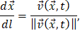
To
enhance computational convenience and efficacy, it is convenient to switch from the time variable
 ,
conventionally the independent variable in ODE systems,

to the path-length variable

|
|
(1)
|
where
 denotes the state vector and
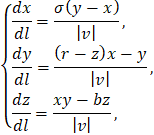
 is the phase velocity. For the Lorenz system, this substitution yields:
|
|
(2)
|
where
 It is crucial to note that system (2) is not equivalent to the original system, as the vector field is now undefined at singular
points coinciding with the fixed points of the Lorenz system:
|

|
(3)
|
This discrepancy,
however, is inconsequential for our purposes, as the lattice is constructed
such that its nodes avoid these singularities. The transition to length-parameterization
is motivated by computational economy, facilitating motion along the trajectory
with a fixed step in length rather than time.
The algorithm for
iterating the discrete trajectory, illustrated in Fig. 1, comprises two stages:
1. A segment of a "continuous" solution (white circles, Fig. 1) of length
L is computed from the initial conditions given by the last point of the
discrete trajectory (black circles, Fig. 1), utilizing a fixed-step numerical
method. The length
 satisfies:
|

|
(4)
|
where
 is the lattice constant,
 is the step size of the numerical method,
 is a positive integer, and
 is a positive real number.
2. The terminal point of the segment is then shifted to the nearest lattice node, which subsequently becomes the next point in the discrete trajectory.
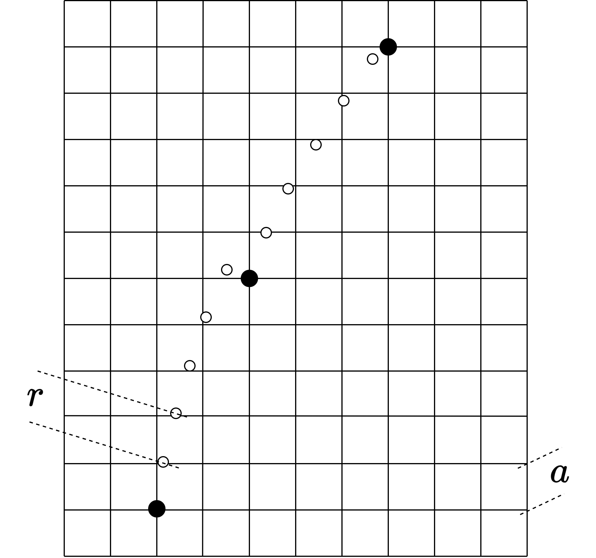
Figure 1. Schematic illustration of the discretization algorithm.
To preclude the
intersection of discrete trajectories with the singular point
 (3), the lattice is
defined to be disjoint from the origin. The procedure for shifting to the
nearest lattice node, incorporating this constraint, is given by:
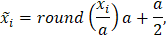
where
 and
 are the coordinates of the segment endpoint and its nearest lattice node, respectively,
and round(x) denotes rounding to the nearest integer.
The parameter
in (3), governing the ratio
 ,
is conventionally termed the "step on the lattice" and, alongside the lattice constant
,
constitutes a pivotal parameter of the algorithm. Although
and
exert a coupled influence on the discretization outcome, their roles can be
heuristically decoupled: the lattice constant a
primarily governs the resolution of the state vector, whereas the step on the lattice
b effectively discretizes the phase velocity vector. Indeed, for a fixed
a, the number of attainable subsequent states is dictated by b; larger
values of b increase the number of potential transitions, yielding smoother discrete trajectories.
In all
experiments reported herein, the 4th-order Runge-Kutta algorithm served as the
computational method.
The
method allows the generation of visualizations for any bounded cross-section of
the phase space pertaining to the dynamical system under investigation. The
results presented in Section 4 were derived exclusively from
two-dimensional cross-sections, which yield 2D images. This restriction was
adopted for two principal reasons. First, the present work does not purport
to offer a systematic investigation of dynamical systems via the proposed
method but is rather devoted to elucidating the method itself. Second, the
application of the method entails substantial computational overhead;
consequently, generating 3D visualizations, videos, or gathering data from
higher-dimensional cross-sections was deemed non-essential within the scope of
this introductory work. What follows is a description of the procedure for
constructing a 2D image using the method of inverse discrete-dissipative
projections.
Consider
a 3-dimensional dynamical system. For the sake of definiteness, let us examine
a region of the phase space defined by


where
 ,
 are constants. We define the visualization lattice within this specified region as:


where
 are positive integer constants, and
is the lattice constant. Our experiments employed a square lattice where
 The set of visualization lattice nodes constitutes a subset of the discretization lattice
nodes or coincides with the latter entirely. The number of visualization
lattice nodes dictates the resolution of the resultant image.
A
cluster comprising the nearest nodes is constructed around each visualization
lattice node (see Fig. 2). In our experiments, the cluster was defined as a
cube with an edge length of 9 discretization lattice nodes, centered on the
visualization lattice node.
Figure 2. Construction of clusters (red points) around
visualization lattice nodes (blue points). Discretization lattice nodes are
shown in gray.
Each
cluster is treated as a discrete phase volume, where the node count is
interpreted as the volume's magnitude. Utilizing the method described in the
preceding section, discrete trajectories are computed for the points within
these clusters. At each computational step, the volume of the discrete cluster —
that is, the count of its unique points — is evaluated. In the general case,
discrete trajectories will coalesce, leading to a reduction in the number of
unique points within the cluster. This yields a function describing the
dependence of the unique point count (the discrete phase volume) on the number
of computational steps. Given that one computational step corresponds to the evolution
of the dynamical system's trajectory over a fixed length (up to the lattice step), we obtain,
to a certain approximation, a function representing the phase volume's dependence on trajectory length.
For
all initial visualization lattice nodes, the number of discrete trajectory
computation steps is fixed at a value N, chosen such that all
trajectories are guaranteed sufficient time to reach the discrete attractor,
i.e., one of the cycles. For each functional dependence, the following quantity
is computed:
|
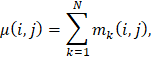
|
(5)
|
where
 is the number of unique points in the cluster defined at the visualization lattice node with coordinates
 (see Fig. 2) after
steps of the discretization method. Finally, we assign to each visualization lattice node
with coordinates
within the selected region its corresponding value
 .
Mapping the
values to colors according to a specified color palette (see the next section) yields the final
image. Thus, each point in the image generated by the method of inverse
discrete-dissipative projections encodes information about the evolutionary
character of a bundle of trajectories emanating from the vicinity of the
corresponding point in the dynamical system's phase space.
The constant N in (5) is determined empirically, and its value can be
established via one of two approaches. Both require the computation of a
discrete trajectory for each visualization lattice node. The first approach
halts computations upon the trajectory's entry into a cycle; the second, upon
its closure. This approach requires prior knowledge of the complete set
of cycles (cf. [2]). Although simpler to implement, the second approach may
require considerable redundant computation, performed after the trajectory has
entered a cycle but before it formally closes. We employed the first approach.
It is
noteworthy that the dependencies of the discrete volumes on the number of computational
steps are quite informative in their own right and could be utilized to
construct more sophisticated and detailed characteristics beyond the scalar
quantities defined in (5).
The
results presented in this section were obtained for the modified Lorenz system
(2). The color palette used for visualization is shown in Fig. 3. This palette
comprises 256 colors. The minimum and maximum values of
are mapped to the leftmost (dark blue) and rightmost (dark red) colors of the palette,
respectively.

Figure 3. Color palette used for visualization.
The first set of
images (Figs. 4 and 5) corresponds to the case of non-chaotic dynamics with system
parameters:
 Discretization parameters were:
 .
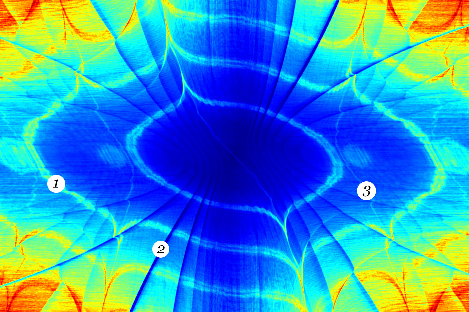
The visualization lattice step was 0.1528. Images (4.A,B,C) represent regions in planes parallel to the
 coordinate plane at
 = 0, 19 and 28.
The region dimensions are
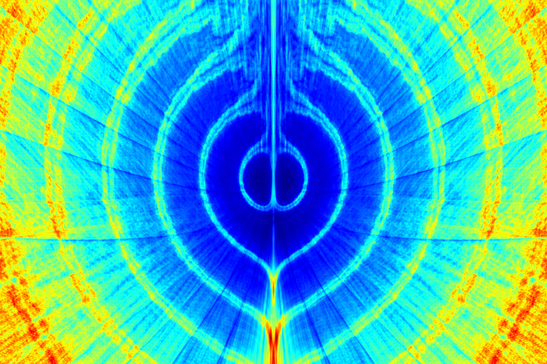
 Fig. 4D shows the visualization for the region
 .
Fig. 5 presents a 3D composite image constructed from regions lying in the coordinate planes
 and the plane
 .
The respective dimensions are indicated on the figure.
Figure 4. Visualization results:
 – cross-sections parallel to the
ΧΥ plane,
 – cross-section in the YZ plane.
A
complex spatial structure is distinctly visible. At least three types of
configurations can be identified (see annotations on Fig. 4A). The first and
most prominent structure 1 partitions the discrete phase space into numerous
cells of non-trivial topology. Furthermore, the boundaries between these cells
are characterized by significantly higher values of the criterion (5) compared
to the cells' interior regions. It will be demonstrated in the subsequent set of
images that this structure loses its sharp boundaries upon the transition to
chaotic dynamics. However, this structure appears to be invariant under refinement of the discretization lattice.
Structure 2, referred to below as "folds," is instead a direct consequence of the applied
discretization algorithm. It will be illustrated below that increasing the
discretization parameter
(step on the
lattice) leads to an increase in the number of these folds. We expect that for large b
the folds should
become visually indistinguishable. Finally, there is structure 3, discernible
as a fine network that occasionally intersects with structure 1. This
structure, while undergoing some modifications, persists upon the transition to
deterministic chaos.
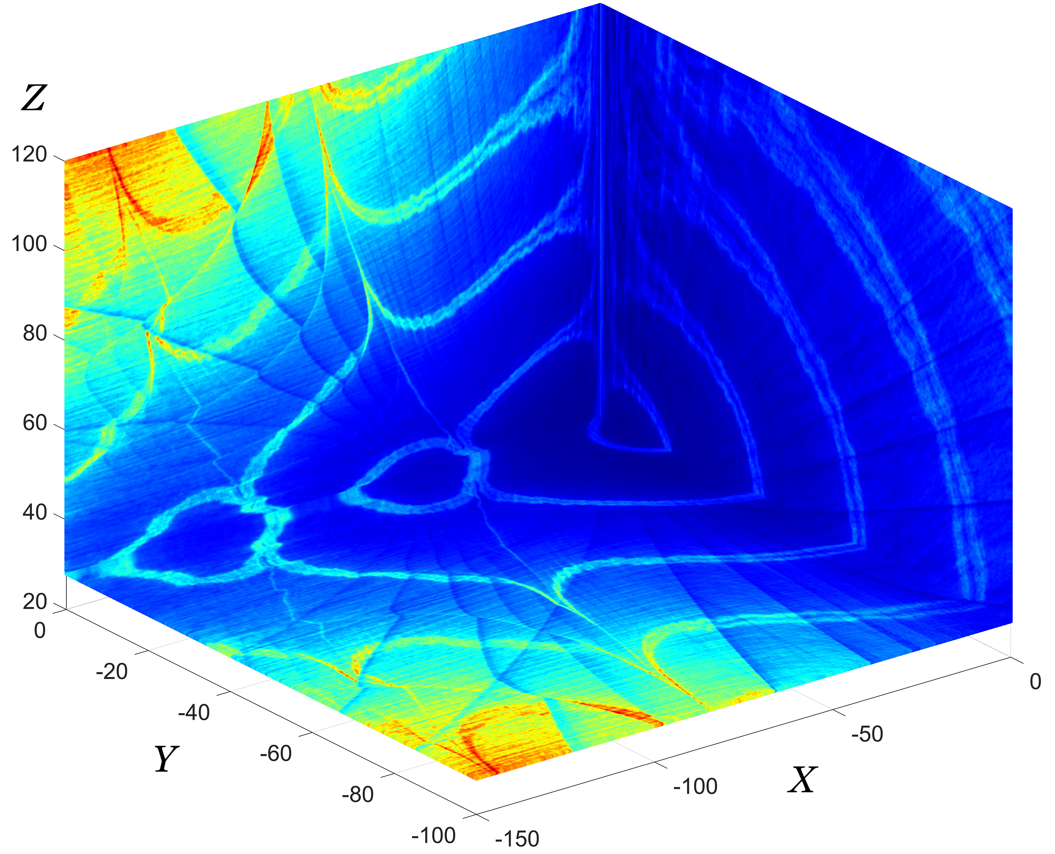
Figure 5. 3D visualization composite for regions lying in the coordinate planes
and the plane
.
Let us
now consider the case of chaotic dynamics under the classical
parameters of the Lorenz system:
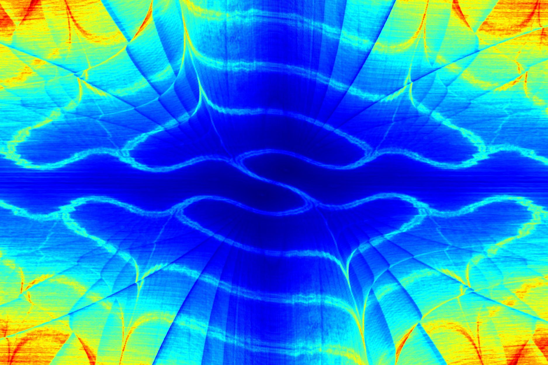
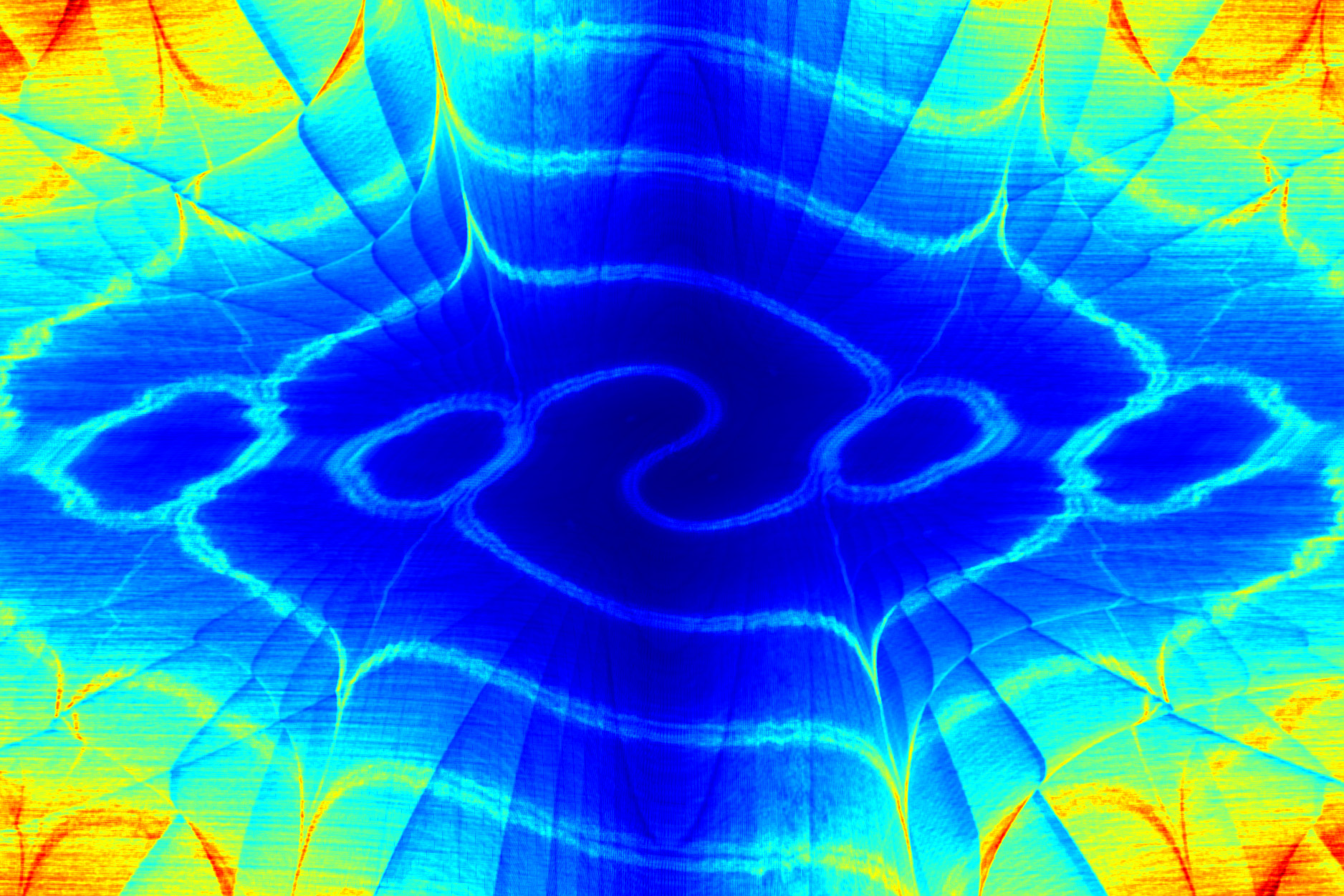
 Figs. 6 and 7 provide illustrations analogous to Fig. 4C,
i.e., for the visualization region
 Figs. 6 and 7 differ in their discretization parameters. For Fig. 6:
 For Fig. 7:
 The visualization lattice step is 0.12 in both cases. Increasing
increases the density of folds. A visualization with discretization parameters
 is virtually identical to that in Fig. 6 and is therefore not shown. This confirms that the
fold density is determined specifically by the parameter

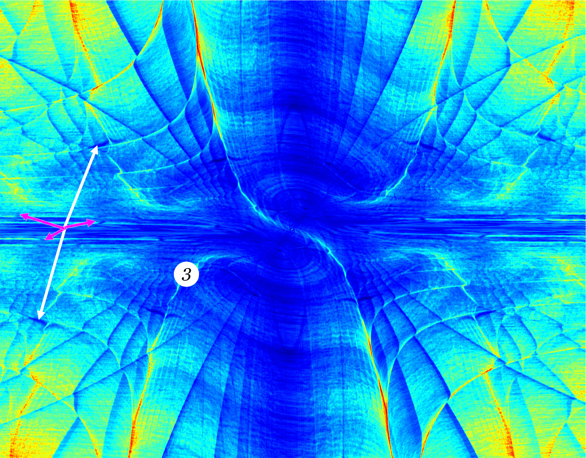
Figure 6. Chaotic dynamics. Visualization region:
Discretization parameters:
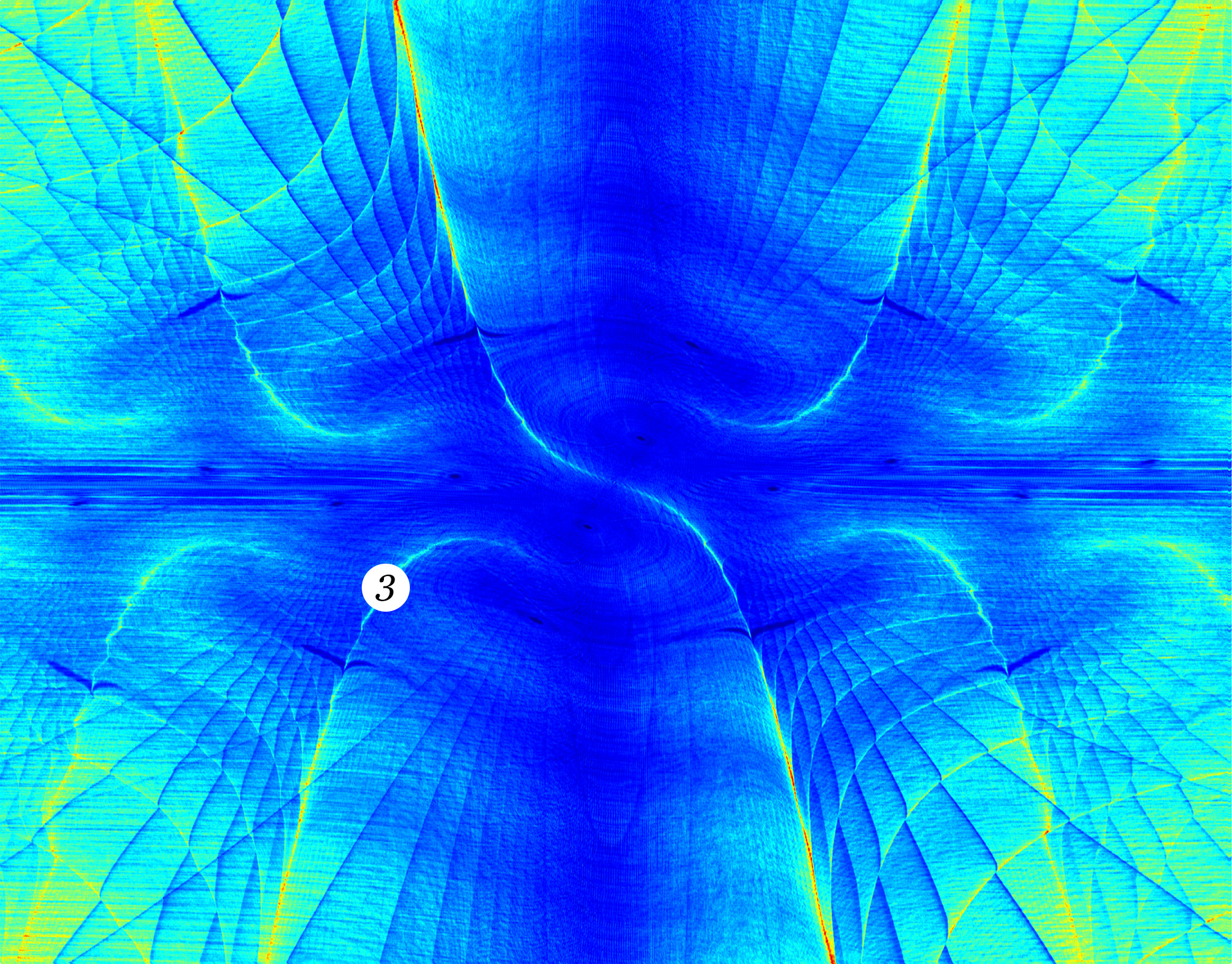
Figure 7. Chaotic dynamics. Visualization region:
Discretization parameters:
Visual analysis of
Figs. 6 and 7, along with other similar images for the chaotic regime,
indicates that structure 1 (Fig. 4A) disintegrate significantly,
leaving behind traces in the form of blurred boundaries. However, structure 3 (Fig. 4A)
persist (see circular markers with the number 3). On the basis of our preliminary results,
we hypothesize that this structure
possesses an invariant component with respect to the discretization parameters
and thus likely has a counterpart in the original continuous system.
In addition to the
structures considered, areas with anomalously rapid reduction of discrete phase
volumes are visible in Figs. 6 and 7 (indicated by white and pink arrows in
Fig. 6). They are more clearly defined in Fig. 7. It can be demonstrated that
these areas correspond to two spirals terminating in the vicinity of the
attractor's fixed points. Located near these fixed points are trivial cycles –
rings. Thus, it can be asserted that the majority of discrete trajectories
constituting the spirals terminate precisely on these rings. Some rings
may be degenerate, consisting of a single point. The total number of rings can
reach several dozen, but in terms of point count, the rings generally
contribute insignificantly compared to the remaining cycles.
All demonstrated
images were generated using original software written in C++ utilizing the CUDA
framework. The creation of visualization images requires substantial
computational resources, justifying the use of many-core graphics processing
units (GPUs).
Analysis of the
results obtained through the application of the inverse discrete-dissipative
projections method yields insights into the behavioral patterns of discretized
dynamical systems in the vicinity of their attractors. As noted in the
introduction, we invariably deal with such systems when simulating them
algorithmically; thus, the scientific value of this line of inquiry is
evident. Within this context, a set of questions arises, the thorough
investigation of which extends beyond the scope of the present work. However,
one particular set of issues warrants immediate discussion: namely, what is the
nature of the mechanism responsible for the emergence of structure 1
and 3 (Fig. 4), and do they bear any relation to the original mathematical
models?
A defining
characteristic of structures 1 and 3 is the relatively high value of criterion
(5) at their boundaries compared to the values observed within the regions.
Based on the conducted numerical experiments, a plausible hypothesis can be
advanced: in most cases, structures 1 and 3 coincide with the boundaries
separating regions from which trajectories reach the attractor at different
times. A discrete phase volume initiating its evolution precisely on the
boundary between two such regions will, with high probability, split into two
subsets, one of which reaches the attractor sooner than the other.
Consequently, the reduction rate of such a volume will be lower compared to
volumes evolving from within the cells defined by the boundaries of structures
1 and 3. Thus, the visualization method effectively highlights the boundaries
between regions characterized by "divergent" system behavior. An
analogy can be drawn here with the application of filters in convolutional
neural networks, which are used to detect edges separating areas of differing
intensity, color, etc., in images.
Regarding the potential
modification or further development of the method, emphasis should be placed on
refining criterion (5). It is conceivable that defining a more complex
characteristic — for instance, employing various types of filters constructed
upon the functional dependency underlying criterion (5) — could yield more
profound information about the behavior of the dynamical system under
investigation.
A method for visualizing the
structural features of attractor basins in discretized dynamical systems has
been proposed. Numerical experiments were conducted, and their results were
presented, forming the basis for conclusions regarding both the structures
revealed through visualization and the operational specifics of the method
itself. The method was tested on the Lorenz system,
considering two types of attractors: a limit cycle and a strange attractor. The
visualizations reveal complex spatial organizations, including persistent
fine-scale networks and discretization-induced folds, whose properties and
origins were analyzed. The method provides a tool for investigating the
interplay between the inherent properties of continuous dynamical systems and
the artifacts introduced by their necessary discretization for computational
study, opening avenues for further research into the geometric structure of
basins of attraction in algorithmic simulations.
1. Kunin I., Chernykh G.,
Kunin B. Optimal chaos control and discretization algorithms // International
Journal of Engineering Science, Vol. 44, Ь 1Р2, 2006, pp. 59Р66
(doi:10.1016/j.ijengsci.2005.05.006)
2. Chernykh, G. Stable and chaotic modes in discrete dynamic systems (Lorenz attractor and Kropotov-Pakhomov neural network model). PhD thesis in physics and mathematics. St. Petersburg, 2004, 103 p.
3. Yamrom B., Kunin I.,
Chernykh G. Centroidal trajectories and frames for chaotic dynamical systems //
International Journal of Engineering Science, Vol. 41, 2003, pp. 465Р473 (doi: 10.1016/S0020-7225(02)00217-3)
4. Li M., Vitányi
P. An Introduction to Kolmogorov Complexity and Its Applications. Cham:Springer, 2019. 834 p. (doi:10.1007/978-3-030-11298-1)
5. Lorenz E. N.
Deterministic nonperiodic flow // Journal of the Atmospheric Sciences, Vol. 20,
1963, pp. 130Р141 (doi:10.1175/1520-0469(1963)020%3C0130:DNF%3E2.0. CO;2) (https://
journals.ametsoc.org/downloadpdf/view/journals/atsc/20/2/1520-0469 _1963_020_0130_dnf_2_0_co_2.pdf)
6. Datseris G., Wagemakers
A. Effortless estimation of basins of attraction // Chaos, Vol. 32, Ь 2, 2022,
023104 (doi:10.1063/5.0076568)
7. Xiong A., Sprott J. C.,
Lyu J., Wang X. 3D Printing С The Basins of Tristability in the Lorenz System
// International Journal of Bifurcation and Chaos, Vol. 27, Ь 8, 2017, 1750128
(doi:10.1142/S0218127417501280) (https://sprott.physics.wisc.edu/pubs/paper 477.htm)
8. Daza A., Wagemakers A.,
Sanjuán M. A., Yorke J. A. Testing for Basins of Wada // Scientific
Reports, Vol. 5, 2015, 16579 (doi:10.1038/srep16579)
9. Ray A., Pal A., Ghosh
D., Dana S. K., Hens C. Mitigating long transient time in deterministic systems
by resetting // Chaos, Vol. 31, Ь 1, 2021, 011103 (doi:10.1063/ 5.0038374)
10. Schultz P., Hellmann
F., Webster K. N., Kurths J. Bounding the first exit from the basin:Independence times and finite-time basin stability // Chaos, Vol. 28, Ь 4, 2018,
043102 (doi:10.1063/1.5013127)
11. van Kan A., Jegminat
J., Donges J. F., Kurths J. Constrained basin stability for studying transient
phenomena in dynamical systems // Physical Review E, Vol. 93, Ь 4, 2016, 042205
(doi:10.1103/PhysRevE.93.042205)
12. Soliman M. S., Thompson
J. M. T. Integrity measures quantifying the erosion of smooth and fractal
basins of attraction // Journal of Sound and Vibration, Vol. 135, Ь 3, 1989, pp.
453-475 (doi:10.1016/0022-460X(89)90699-8)
13. Rega G., Lenci S.
Dynamical Integrity and Control of Nonlinear Mechanical Oscillators // Journal
of Vibration and Control, Vol. 14, Ь 1-2, 2008 (doi:10.1177/1077546307079403)
14. Zhai C., Nguyen H. D.
Estimating the Region of Attraction for Power Systems Using Gaussian Process
and Converse Lyapunov Function // IEEE Transactions on Control Systems
Technology, Vol. 30, Ь 3, 2022, pp. 1328-1335 (doi:10.1109/TCST.2021. 3098167)
15. Mohammadi H., Peet M.
M. Estimating the Region of Attraction Using Polynomial Optimization: a
Converse Lyapunov Result // arXiv preprint arXiv:1704.06983, 2017
(https://arxiv.org/abs/1704.06983)
16. Liu J., Meng Y.,
Fitzsimmons M., Zhou R. Towards Learning and Verifying Maximal Neural Lyapunov
Functions // 2023 62nd IEEE Conference on Decision and Control (CDC), Singapore,
Singapore, 2023, pp. 8012-8019 (doi:10.1109/CDC49753.2023. 10383299)
17. Shadden S. C., Lekien
F., Marsden J. E. Definition and properties of Lagrangian coherent structures
from finite-time Lyapunov exponents in two-dimensional aperiodic flows // Physica
D: Nonlinear Phenomena, Vol. 212, Ь 3-4, 2005, pp. 271-304
(doi:10.1016/j.physd.2005. 10.007)
18. Darriba L. A., Maffione
N. P., Cincotta P. M., Giordano C. M. Comparative study of variational chaos
indicators and ODEs' numerical integrators // International Journal of
Bifurcation and Chaos, Vol. 22, Ь 10, 2012, 1230033
(doi:10.1142/S0218127412300339)
19. García-Garrido
V. J., García-Luengo J. Painting the phase space of dissipative systems
with Lagrangian descriptors // Communications in Nonlinear Science and
Numerical Simulation, Vol. 104, 2022, 106034 (doi:10.1016/j.cnsns.2021.106034)
20. Agaoglou M.,
García-Garrido V. J., Katsanikas M., Wiggins S. Visualizing the phase
space of the HeI2 van der Waals complex using Lagrangian descriptors //
Communications in Nonlinear Science and Numerical Simulation, Vol. 103, 2021,
105993 (doi:10.1016/j.cnsns. 2021.105993)
21. Daquin J., Pédenon-Orlanducci
R., Agaoglou M., García-Sánchez G., Mancho A. M. Global dynamics
visualisation from Lagrangian Descriptors. Applications to discrete and
continuous systems // Physica D: Nonlinear Phenomena, Vol. 442, 2022, 133520
(doi:10.1016/j.physd. 2022.133520)
22. Rannou F. Numerical
study of discrete plane area-preserving mappings // Astronomy and Astrophysics,
Vol. 31, 1974, pp. 289Р301 (https://ui.adsabs.harvard.edu/abs/ 1974A%26A.... 31..289R)