BOUNDARY IDENTIFICATION ALGORITHMS AND VISUALIZATION OF THE SOLUTION OF THE PLATEAU PROBLEM IN A BLENDER ENVIRONMENT
E.G. Grigorieva, A.A. Klyachin, V.A. Klyachin
Volgograd State University, Volgograd, Russia
e_grigoreva@volsu.ru, klyachin-aa@yandex.ru, klyachin.va@volsu.ru
Contents
2. Identification of boundary points
4. Visualization of the Plateau problem solution
5. Calculation and 3D modeling of minimal surface areas with a specified overlapping volume
Abstract
In this paper we consider the calculation and construction of the surface having the lowest possible area with the specified edge and the value of the volume of domain that covers this surface. This problem is known from the practice of modern design constructions in which thin shell are often used as coatings or protections. Therefore, one has to solve the problem: How to cover the volume, having a fixed or maximum value, for the minimum area of the its surface. In our work we mathematically formulate this variational problem and present a solution algorithm, using the solutions of the equation of constant mean curvature. The article gives a description of the software implementation of this algorithm, the images calculated surfaces with different computational domain and the boundary conditions. Accuracy of calculations on the average was 0.01%.
For the numerical solution of the classical Plateau problem it was built a mathematical model that allows to reduce the problem of minimizing the corresponding functional of the functional area type to the finite-dimensional case. In order to visualize resulting solutions, we consider the possibility of constructing the boundary contours directly in Blender modeling environment. At the same time, the article demonstrates two algorithms for the identification of such circuits for multi-faceted surfaces of an arbitrary topological structure. The implementation of the mentioned algorithms in the simulation environment allows us to calculate of the surface with a minimum value of the functional in interactive mode, and the calculation results are stored in a convenient 3D format. Currently, the built-in module is placed in the public domain on GitHub server and includes the implementation of algorithms for the calculation of minimal surfaces, the capillary surfaces and surfaces of constant mean curvature.
Keywords: surface of minimal area, space triangulation, piecewise linear surface, approximation of the area functional, constant mean curvature surface, capillar surface.
1. Introduction
In the practice of designing modern structures, thin shells are often used as coatings or enclosures [10], [11]. In connection with this, the actual problem is how to cover a volume with a fixed or maximum value with the smallest area of the shell. The solution allows to minimize material consumption and shell weight at the maximum cubic capacity of the structure. As noted in [10], "Nature constructs in the form of a soap film the only possible uniformly strained equilibrium shape with a fixed subshell volume and minimum surface area for a given external load.The relative geometric parameters of the shape of the surfaces of soap films can be taken as optimal parameters that should be taken into account when designing real air cushions of an air-bearing type. "In addition, we add that the minimal surfaces themselves have an attractive appearance.This solution of the problem is divided into two main case: the case of parametric surfaces of an arbitrary topological structure and the case of nonparametric surfaces given by a graph of a suitable function. In the first case, minimization of the area type functional is carried out using the gradient descent method in the class of piecewise linear surfaces with a fixed boundary that is a three-dimensional polygonal line. A particular case of the problem being solved is the classical Plateau problem [3], [4] for minimal surfaces. The topology of the desired surface is set visually by building its model in the 3D editor. This requires solving the problem of defining boundary vertices, so that it is possible to construct a boundary polygonal line. In our work, we describe two algorithms for solving this problem. Minimization of functionals for constructing equilibrium surfaces is illustrated by the example of classes of minimal surfaces, surfaces of constant mean curvature, tents, and capillary surfaces. We note several papers devoted to software modeling of minimal surfaces of different topological structures [16], [17], [18].
For graphs, the problem reduces to finding solutions to the equation of constant mean curvature. The Dirichlet problem for this equation has been investigated by many mathematicians. One of the first papers in which the existence and uniqueness theorems for solutions of this problem were obtained are the papers [14], [15]. To find approximate solutions, we use a variational method that involves minimizing some integral functional in the class of piecewise linear functions. In our article we describe the algorithm and its software implementation of the calculation of such surfaces based on the corresponding mathematical model.
The paper deals with the problem of constructing a surface having the smallest possible area, provided that such a surface overlaps the volume of a fixed value. Several software modules have been developed that allow calculating such surfaces and processing the obtained data to construct its three-dimensional model.
2. Identification of boundary points
When solving computational problems in domains of complex
shape (for example, in problems of calculating the shape of equilibrium
surfaces [1], [2]), initialization of boundary conditions becomes especially
laborious if the corresponding computational grid has a significantly large
number of nodes. Note that modeling such areas and surfaces is not difficult if
you use the editor of geometric models. In particular, the Blender package provides
an opportunity to design a model of a design area and an arbitrary-shaped
surface. However, the determination of the boundary vertices of the model is
possible only for each component of the boundary connectivity in the manual
mode. In this article we present some algorithms for solving such a problem.
Let us give a formal description. Let ![]() be an arbitrary a polyhedral surface in
three-dimensional space. Such a surface can be defined by means of two finite
sets (arrays). At first, it is a set V of vertices of surface M.
The corresponding array has the form
be an arbitrary a polyhedral surface in
three-dimensional space. Such a surface can be defined by means of two finite
sets (arrays). At first, it is a set V of vertices of surface M.
The corresponding array has the form
![]()
Secondly, it is a set of T triangular faces of a polyhedral surface, which can be specified by an array of the form
![]()
In this array, the numbers are the numbers of points from
the array V that are the vertices of the corresponding triangle. The problem is
posed as a problem of determining an array B of numbers of those vertices of
V that are boundary points in the sense of the usual topology of continuous
surfaces in![]() .
Each algorithm we consider at its first step constructs a triangulation
of each face of a polyhedral surface and an auxiliary array NT of the form
.
Each algorithm we consider at its first step constructs a triangulation
of each face of a polyhedral surface and an auxiliary array NT of the form
![]() ,
,
where NT [k] is an array of numbers of triangles from the
array T for which the point V [k] is a vertex. In other words, for each vertex ![]() there is a list of
triangles incident to this vertex. The first of the considered algorithms counts
the number f (k) of faces and the number e (k) of edges incident to the vertex
there is a list of
triangles incident to this vertex. The first of the considered algorithms counts
the number f (k) of faces and the number e (k) of edges incident to the vertex ![]() . If we denote
by | | capacity of the set, then the indicated quantities are defined as
follows f(k)=|NT[k]|, e(k)=|E(k)|, where
. If we denote
by | | capacity of the set, then the indicated quantities are defined as
follows f(k)=|NT[k]|, e(k)=|E(k)|, where ![]() . Then condition e(k)=f(k) is
necessary and sufficient for the vertex
. Then condition e(k)=f(k) is
necessary and sufficient for the vertex ![]() was not a boundary value. The second algorithm
is based on counting the number of occurrences of vertices in triangles
incident to a given vertex. For this purpose, for each vertex
was not a boundary value. The second algorithm
is based on counting the number of occurrences of vertices in triangles
incident to a given vertex. For this purpose, for each vertex ![]() a set is constructed (the
multiplicity of occurrences of elements is assumed)
a set is constructed (the
multiplicity of occurrences of elements is assumed) ![]()
The boundary condition of a point, in this case, is
equivalent to the fact that at least one number in ![]() will be unique.
will be unique.
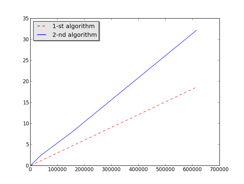
Fig. 1. Comparison of algorithms for identification of boundary points.
The algorithms are implemented as an embedded module in the Blender 2.77 programming environment in the Python 3 programming language. This module allows you to calculate the boundary of an arbitrary polygonal model located in the 3D view window using the interface generated by this module and built into the Blender environment. The calculation result can be saved as a standard format file for spatial models, which in turn can be used to initialize the boundary conditions. The graph below shows the experimental data of the execution time of the implementations of the above algorithms. The horizontal axis indicates the number of faces of the models in question, and along the vertical axis - the time of the boundary calculation in seconds. Comparison shows that the first algorithm is approximately 1.5 times faster than the second one.
Further, we demonstrate the use of the obtained algorithm as the numerical solution of the classical Plateau problem of finding the surface of a minimal area that tightens a given contour in space.
3. The Plateau problem
The classical boundary value problem of geometry is the
so-called Plateau problem. This task consists in constructing the surface of
the minimal area with a given edge. In the two-dimensional case, the existence
of a solution to the Plateau problem was proved by Douglas and Radot [3], [4].
We consider the numerical solution of this problem by the method of
gradient descent in a special constructed space. Let as above the polyhedral
surface ![]() is
given by a set of V points and an array of triangles T. For each integer N and
the array T one can construct a linear space
is
given by a set of V points and an array of triangles T. For each integer N and
the array T one can construct a linear space ![]() elements of which will be polyhedral
surfaces with N vertices and faces defined by the array T. The operations of
addition and multiplication by a number in
elements of which will be polyhedral
surfaces with N vertices and faces defined by the array T. The operations of
addition and multiplication by a number in ![]() are introduced in a natural way as vector
operations on an array of points V. At the same time, an array T is preserved,
along which the faces of the surface are defined. The points of such a space
will be denoted by a capital Latin letter, and the corresponding tops of the
surface by capital letters
are introduced in a natural way as vector
operations on an array of points V. At the same time, an array T is preserved,
along which the faces of the surface are defined. The points of such a space
will be denoted by a capital Latin letter, and the corresponding tops of the
surface by capital letters![]() . We denote by
. We denote by ![]() the set of triangles of the corresponding
polyhedral surface. We consider the functional
the set of triangles of the corresponding
polyhedral surface. We consider the functional
![]() ,
,
where the sum is taken over all triangles ![]() and f(S) is a
certain positive function on the set of all triangles. In [5], a functional
constructed from the function
and f(S) is a
certain positive function on the set of all triangles. In [5], a functional
constructed from the function![]() , where
, where ![]() is a positive homogeneous of degree 1, convex
down function, but
is a positive homogeneous of degree 1, convex
down function, but ![]() is a normal to the plane of the triangle
is a normal to the plane of the triangle ![]() . It was assumed
that
. It was assumed
that![]() , which
means that the value of the functional F is independent of the orientation of
the surface. Nevertheless, we assume that the surfaces in question are oriented.
For such a functional, a gradient was calculated in [5]
, which
means that the value of the functional F is independent of the orientation of
the surface. Nevertheless, we assume that the surfaces in question are oriented.
For such a functional, a gradient was calculated in [5]
![]() ,
,
where the sum over all triangles S incident to the
vertex![]() ,
, ![]() is a vector
connecting the vertices of the triangle S that do not coincide with the vertex
is a vector
connecting the vertices of the triangle S that do not coincide with the vertex ![]() . In this case, the
triangles are traversed in accordance with the positive orientation of the
surface. Note that the vector
. In this case, the
triangles are traversed in accordance with the positive orientation of the
surface. Note that the vector ![]() formally can be regarded as a vector of space
formally can be regarded as a vector of space ![]() . Therefore, to find
the minimum of the functional F, we use the method of gradient descent. This
method is an iterative process view
. Therefore, to find
the minimum of the functional F, we use the method of gradient descent. This
method is an iterative process view
![]() ,
,
where the amount of displacement ![]() can be chosen experimentally. In this
case, you must specify
can be chosen experimentally. In this
case, you must specify ![]() . This point will specify the initial shape of
the surface, and during the calculation its edge must be fixed. This is
achieved by calculating the gradient
. This point will specify the initial shape of
the surface, and during the calculation its edge must be fixed. This is
achieved by calculating the gradient![]() by the above formula at all points, with the
exception of boundary points, in which the value
by the above formula at all points, with the
exception of boundary points, in which the value ![]() is assumed to be zero. In the present
work we consider the case
is assumed to be zero. In the present
work we consider the case ![]() , which corresponds to piecewise-linear minimal
surfaces. In this case
, which corresponds to piecewise-linear minimal
surfaces. In this case
![]() .
.
4. Visualization of the Plateau problem solution
To visualize the solution of the Plateau task, an embedded
module was developed in the Blender 2.7 environment. This module is a package
consisting of program modules in the programming language Python. The package
structure includes five files. Files geometry.py and triangulation.py contain
classes for calculating the geometric characteristics of triangles and
piecewise linear surfaces in ![]() . In a file ndimvar.py
a generalized gradient descent algorithm was implemented. A file minsquare.py contains
calculating the gradient of the area functional for piecewise linear surfaces
in
. In a file ndimvar.py
a generalized gradient descent algorithm was implemented. A file minsquare.py contains
calculating the gradient of the area functional for piecewise linear surfaces
in![]() . All
geometric data classes are based on NumPy arrays. This package became available
in the Blender environment, starting with version 2.7. The last file of package panel_addon.py
implements an interface for the user of the program. The interface offers
three functions:
. All
geometric data classes are based on NumPy arrays. This package became available
in the Blender environment, starting with version 2.7. The last file of package panel_addon.py
implements an interface for the user of the program. The interface offers
three functions:
1. Drawing the border of the selected object in the 3D view window.
2. Setting the number of iterations and step![]() of the gradient descent
method.
of the gradient descent
method.
3. Calculation of the surface obtained by applying a specified number of iterations to the selected object.
In this case, as the contour in the corresponding Plateau
problem, the boundary of this selected object is selected. To use the package,
you need to put the files in the / scripts / addons directory in the Blender
installation directory. At the next program loading the package will be added
to the list of available plug-ins that the user can see through the main
program menu File->User Preference->Addons->3D View.
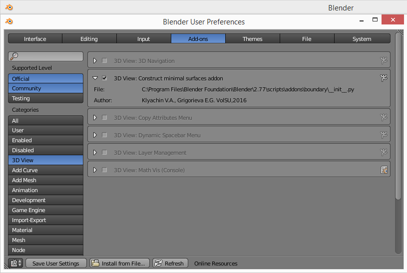
Fig. 2. Display information about the connected module in the Blender environment.
After marking this module, it becomes available for use through the designed interface.
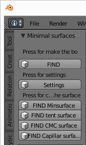
Fig. 3. The graphical interface provided by the built-in module.
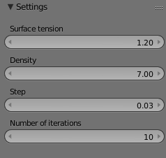
Fig. 4. Configuring the module settings.
The module implements algorithms for calculating not only minimal surfaces, but also surfaces with constant average curvature (Constant Mean Curvature surfaces), tent surfaces (minimizing the potential energy of a heavy elastic surface), and a capillary surface. For calculation, the user interface built into the Blender program allows defining parameters such as the density of the liquid medium, its surface tension coefficient, the value that determines the step of iterating the gradient descent, and the number of iterations of the algorithm.
Below is the result of the search for boundary edges of a surface modeled in the 3D view of the Blender program.
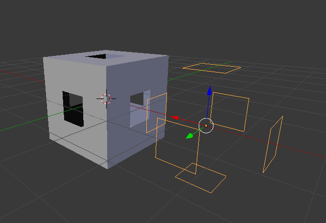
Fig. 5. The result of the algorithm for identifying the boundary.
To solve the variational problem, it is first necessary to construct a computational grid on the surface. You can perform this operation in edit mode with the Blender Subdivide tool. Triangulation of the grid is also performed by standard Blender tools using the Triangulation modifier.
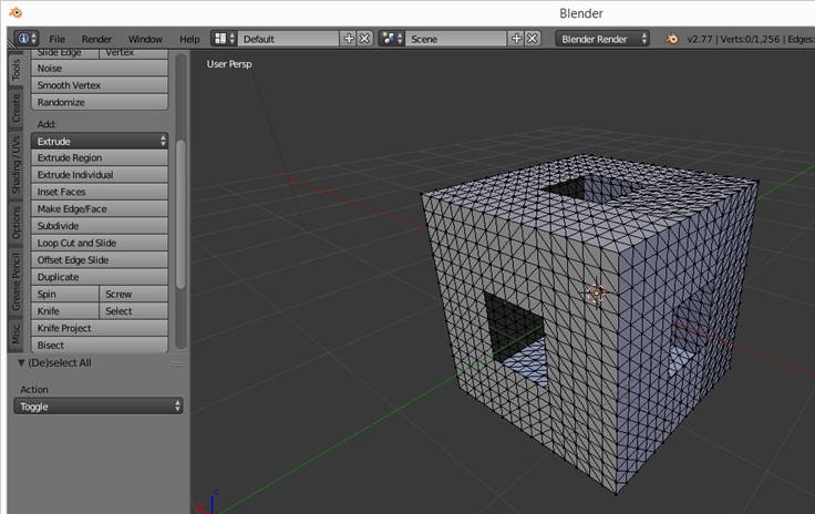
Fig. 6. Triangulation of the model surface.
Below is a visualization of the process of minimizing the surface area by the method of gradient descent. A total of 750 iterations were performed. Each GIF frame was created after 50 iterations. Figure 7 shows that the iterative process smooths the corners of the cube, as the points of convexity of the initial surface. This fact agrees with the theoretical conclusions about the fact that each point of the minimal surface is a saddle point or a hyperbolic point with Gaussian curvatureK<0.
Fig. 7. Visualization of the process of gradient descent.
The next GIF animation shows the situation when the cylinder is pulled into a segment that connects the centers of two circles that are in two parallel planes at a sufficient distance. This is because the corresponding Plateau problem in this case has no solution in the class of surfaces of revolution. Theoretical grounds for this effect are given in [6] - [9].
Fig. 8. By retaining the topological type of surface, the minimization process tends to get two disks.
We give some more minimal surfaces with a boundary contour having a complex geometric structure and calculated using the module developed by us. It should be noted that 750 iterations of the gradient descent method were used to obtain an established surface shape, as above.
Fig. 9. Visualization of minimal surfaces calculated by the method of gradient descent.
Below in Fig. 10, visualization of the result of calculation of almost periodic minimal surfaces is given. The first model is obtained using the principle of symmetry, which allows the surface to be distributed unrestrictedly into the whole space.

Fig. 10. Example of visualization of a fragment of periodic minimal surfaces.
The result of modeling a capillary surface is presented in the next GIF animation (see Figure 11). Here one can observe the process of formation of the shape of a drop of liquid in the field of gravity.
Fig. 11. The process of modeling the drop.
The module developed by us is freely available at github.com by address:
https://github.com/KlyachinVA/MinimalSurface
To connect it to the Blender environment, you need to download the zip-archive from the specified address, and unpack it into the scripts / addons / boundary directory in the installation directory of the Blender package.
5. Calculation and 3D modeling of minimal surface areas with a specified overlapping volume
In this section of the paper, we consider the problem of
finding a surface that has the smallest possible area for a given value of the
volume that it overlaps. The problem is formulated mathematically as follows.
Let on the plane ![]() with Cartesian coordinates
with Cartesian coordinates ![]() a bounded domain
a bounded domain ![]() is given and
is given and ![]() is a continuous
function defined in the closure of this domain. It is required for a fixed
positive number
is a continuous
function defined in the closure of this domain. It is required for a fixed
positive number ![]() to
define a function
to
define a function ![]() such that
such that
wherein
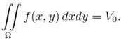 (2)
(2)In our work we solve this problem in the class of piecewise linear surfaces, that is, surfaces composed of triangles adjacent to each other. It is known that the solution of this variational problem will satisfy a nonlinear differential equation with partial derivatives
with the boundary condition
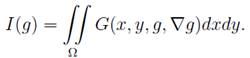
The constant value of H, which is equal to the average curvature of the graph f (x, y), is determined by the value of the overlapped volume.It is not possible to find the exact solution of a given boundary-value problem most often. In this paper we use an approach that involves the construction of approximate solutions of equation (3) over an arbitrary domain with a given triangulation. To calculate such surfaces and further processing of the obtained data, we developed a computational program for the approximate solution of variational boundary value problems for a functional of general form
For our task, we took ![]() . With its help, the surfaces of the
minimum area with a given value of the volume overlapped by them and with different
boundary conditions were calculated. To build surfaces and their images, we
saved the results of calculations in a text file of the STL format and used the
Blender 2.67b program. In this paper, we present images of some of the surfaces
constructed. Note that the developed program allows you to find an
approximately necessary surface over an area of a complex
shape. This is achieved since that the main condition for carrying
out the calculations is the presence of three input files that contain a list
of vertices and triangles of triangulation, as well as the values of the
boundary function.This achieves the universality of the program and its
independence from the structure of the calculated grid. We note that in [12],
the problem of constructing minimal surfaces without additional conditions on
volume was solved in a similar way.
. With its help, the surfaces of the
minimum area with a given value of the volume overlapped by them and with different
boundary conditions were calculated. To build surfaces and their images, we
saved the results of calculations in a text file of the STL format and used the
Blender 2.67b program. In this paper, we present images of some of the surfaces
constructed. Note that the developed program allows you to find an
approximately necessary surface over an area of a complex
shape. This is achieved since that the main condition for carrying
out the calculations is the presence of three input files that contain a list
of vertices and triangles of triangulation, as well as the values of the
boundary function.This achieves the universality of the program and its
independence from the structure of the calculated grid. We note that in [12],
the problem of constructing minimal surfaces without additional conditions on
volume was solved in a similar way.
To solve the problem (1),
(2)
for a given value of the mean curvature H we solve the boundary
value problem (3), (4).
For this we use the variational method for finding such a function ![]() , on which the
functional reaches its minimum value
, on which the
functional reaches its minimum value
![]()
among all functions ![]() such that
such that ![]() In what follows we assume that the domain
In what follows we assume that the domain ![]() is a polygon
in the plane. Consider a partition of this polygon into nondegenerate triangles
is a polygon
in the plane. Consider a partition of this polygon into nondegenerate triangles
![]() . Let
. Let ![]() be all vertices of
these triangles. We assume that none of the points
be all vertices of
these triangles. We assume that none of the points ![]() not an internal point of any side of
the triangles. This construction will be called the triangulation of the domain
not an internal point of any side of
the triangles. This construction will be called the triangulation of the domain
![]() and
denote
and
denote ![]() . Next,
we call the fineness of the partition the quantity
. Next,
we call the fineness of the partition the quantity ![]()
For an arbitrary set of numerical values ![]() we define a piecewise
linear function
we define a piecewise
linear function ![]() so
that
so
that ![]() and
function
and
function ![]() on
each triangle
on
each triangle ![]() .
This function will be continuous in
.
This function will be continuous in ![]() and in each triangle
and in each triangle ![]() gradient definition
gradient definition ![]() .Therefore, we can
calculate the value of the functional
.Therefore, we can
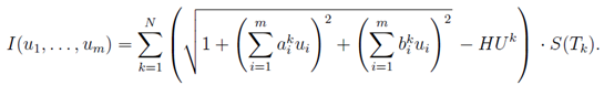
calculate the value of the functional ![]() for a piecewise-linear function
for a piecewise-linear function ![]()

where ![]() -- area of a triangle
-- area of a triangle ![]() ?
? ![]() -- arithmetic average of function values
-- arithmetic average of function values ![]() in vertices of
a triangle
in vertices of
a triangle ![]() . Values
of variables
. Values
of variables ![]() are
expressed linearly in terms of the variables
are
expressed linearly in terms of the variables ![]() . Then there exist numbers
. Then there exist numbers ![]() and
and ![]() , sch that
, sch that
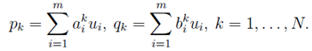
Coefficients ![]() and
and ![]() are uniquely determined by a partition of the
domain
are uniquely determined by a partition of the
domain ![]() on triangles
on triangles ![]() .
Therefor
.
Therefor
We pose the problem of finding such a piecewise linear
function ![]() ,
on which the minimum of the functional is attained
,
on which the minimum of the functional is attained ![]() , that is, the problem
, that is, the problem
![]()
where the minimum is sought among all the sets ![]() , for which
, for which ![]() .
.
To solve the problem (3)
- (4)
we used a simple gradient method to find the minimum points of functions of a
finite number of variables. For this purpose, we developed the basic procedure
for minimizing minimum_func_mix() and several auxiliary, necessary for the
preparation of calculations. Briefly describe their work. Note first that the
coordinates of the nodes of the triangulation ![]() are stored in a separate file having a
simple structure: the first 8 bytes are allocated to the number of these
points, and then each point occupies 20 bytes - two coordinates of 8 bytes and
information about the boundary membership and the type of the boundary condition
(4 more bytes). We also note that in the function minimum_func_mix() the
possibility of specifying both the Dirichlet boundary conditions, that is, the
values of the desired solution on the boundary of the domain, and mixed
boundary conditions containing the conditions on the derivatives of this
solution, is realized. Here in these 4 bytes we specify the type of the point:
0 - the inner point of the region
are stored in a separate file having a
simple structure: the first 8 bytes are allocated to the number of these
points, and then each point occupies 20 bytes - two coordinates of 8 bytes and
information about the boundary membership and the type of the boundary condition
(4 more bytes). We also note that in the function minimum_func_mix() the
possibility of specifying both the Dirichlet boundary conditions, that is, the
values of the desired solution on the boundary of the domain, and mixed
boundary conditions containing the conditions on the derivatives of this
solution, is realized. Here in these 4 bytes we specify the type of the point:
0 - the inner point of the region ![]() , 1 is a boundary point with the Dirichlet
condition, 2 is the boundary point at which the condition on the derivatives of
the solution is given.
, 1 is a boundary point with the Dirichlet
condition, 2 is the boundary point at which the condition on the derivatives of
the solution is given.
The triangles of the used triangulation are also included in a separate file, which is arranged in a similar way: first, 8 bytes are assigned to the total number of triangles, then the numbers of the points making up the described triangle go. Thus, for each triangle we allocate 24 bytes (three points numbers of 8 bytes).
As mentioned above, we solve the problem in the class of
piecewise-linear functions. Any such function defined over the domain ![]() is uniquely
determined by its values at the nodes of the triangulation. Therefore, we store
the piecewise linear function in files in which the first 8 bytes are occupied
by the number of triangulation points, and then the function values in the
corresponding vertices go sequentially.
is uniquely
determined by its values at the nodes of the triangulation. Therefore, we store
the piecewise linear function in files in which the first 8 bytes are occupied
by the number of triangulation points, and then the function values in the
corresponding vertices go sequentially.
Gradient method involves the calculation of derivatives ![]() for those values of the
index i for which the point
for those values of the
index i for which the point ![]() is internal for the region
is internal for the region ![]() . Then
after differentiating expression I in
. Then
after differentiating expression I in ![]() in the corresponding sum there will remain terms
only for those triangles that contain a point
in the corresponding sum there will remain terms
only for those triangles that contain a point ![]() as its vertex. Therefore, to increase
the speed of the program, we create a structure in which for each triangulation
node a set of triangles adjacent to this point is stored.
as its vertex. Therefore, to increase
the speed of the program, we create a structure in which for each triangulation
node a set of triangles adjacent to this point is stored.
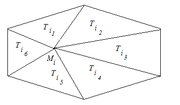
Fig. 12. Neighboring triangles for the vertex ![]() .
.
Then, after completely natural transformations, the
computational scheme will look like this. If the index ![]() denote the iteration
number, then in step
denote the iteration
number, then in step ![]() values in internal nodes
values in internal nodes ![]() triangulations are recalculated by
formula
triangulations are recalculated by
formula
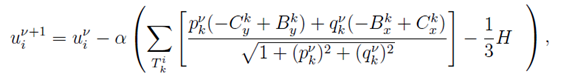
where the summation is taken over the triangles ![]() , whose
points
, whose
points ![]() is
the vertex, and
is
the vertex, and ![]() and
and
![]() two other
points of the triangle
two other
points of the triangle ![]() ,
, ![]() -- step gradient descent.
-- step gradient descent.
Thus, for each value of H we find an approximate solution
of the boundary-value problem (3), (4)
in the form of values ![]() in nodes of triangulation
in nodes of triangulation ![]() . These values uniquely
determine a piecewise linear function
. These values uniquely
determine a piecewise linear function ![]() . If we now calculate the integral
. If we now calculate the integral
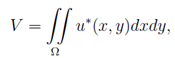
then a continuous function V=V(H) is defined. To
solve the initial problem (1)-(2)
at a given ![]() it
is enough to find such
it
is enough to find such![]() , that
, that ![]() . For this, we proceed according to the
following algorithm:
. For this, we proceed according to the
following algorithm:
1) we find the segment ![]() such that the number
such that the number ![]() falls between the values
falls between the values ![]() and
and ![]() ;
;
2) let ![]() . Then, if
. Then, if ![]() , then we consider the segment
, then we consider the segment ![]() and further we assume
and further we assume ![]() . If
. If ![]() , then we consider the
segment
, then we consider the
segment ![]() and
further we assume
and
further we assume ![]() . If
. If ![]() , then the desired point was found and we assume
, then the desired point was found and we assume
![]() ;
;
3) then we act in accordance with the method of dividing the
segment in half, repeating step 2), and with the necessary accuracy we find ![]() .
.
The calculation results are the approximate values found ![]() , corresponding to
the minimum point of the function I. These values are stored in a
separate file, the description of which we gave above. We have also written a
procedure for the final processing of the calculation results, which converts
them into two types of files. One of them is a text file, each line of which
stores three-dimensional coordinates of one point of the model. Three
consecutive lines specify one triangle in the triangulation of the surface.
Another file is a standard stl graphics file stl for storing such a surface.
, corresponding to
the minimum point of the function I. These values are stored in a
separate file, the description of which we gave above. We have also written a
procedure for the final processing of the calculation results, which converts
them into two types of files. One of them is a text file, each line of which
stores three-dimensional coordinates of one point of the model. Three
consecutive lines specify one triangle in the triangulation of the surface.
Another file is a standard stl graphics file stl for storing such a surface.
In the beginning, we checked the calculation accuracy using the example of constructing a circular cylinder over a rectangular region. It is known that such a surface has a constant average curvature equal to the reciprocal of the radius of the base of the cylinder. Therefore, knowing this exact solution, it is not difficult to estimate the degree of error in calculations.
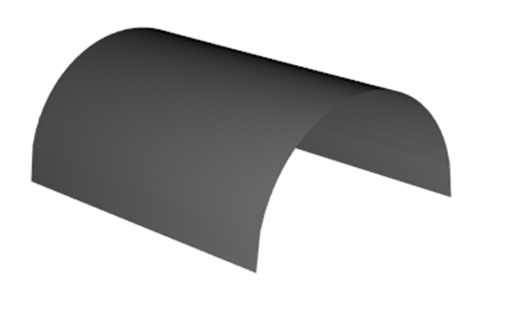
Fig. 13. Cylindrical surface.
For 2500 knots of triangulation, the accuracy of the calculations turned out to be on the order of 0.1%. We note that the convergence of the applied method was previously studied in [2], [12] and for the equation of the minimal surface and the equation of the equilibrium capillary surface. For the constant mean curvature equation, which we use to calculate our surfaces, we can prove the same property of convergence by the same methods.
A series of experiments was then carried out with different
values of H and boundary functions ![]() . For example, in order to see how the
surface shape changes depending on the average curvature, and therefore the
overlap volume, the calculations were made for the following values of H:
from 0 to 1.9 in increments of 0.1. The image of four of the resulting surfaces
is shown in Figure 11.
. For example, in order to see how the
surface shape changes depending on the average curvature, and therefore the
overlap volume, the calculations were made for the following values of H:
from 0 to 1.9 in increments of 0.1. The image of four of the resulting surfaces
is shown in Figure 11.
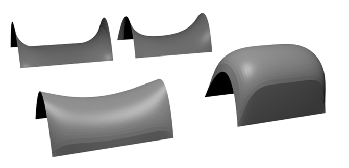
Fig. 14. Dynamics of change in the shape of the surface, depending on the value of the average curvature.
In the following pictures, we placed images of some of the calculated surfaces above the rectangular and octagonal areas. For them, a triangulation was used, the description and study of the quality of which was given in work [13].
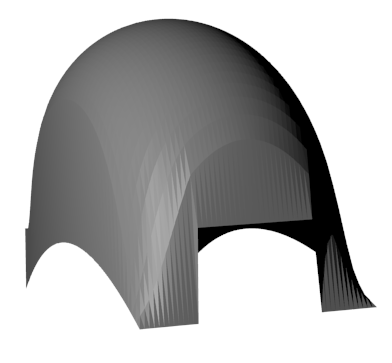
Fig. 15. Surface with a parabolic boundary skeleton over a rectangular area (H = 1.0).
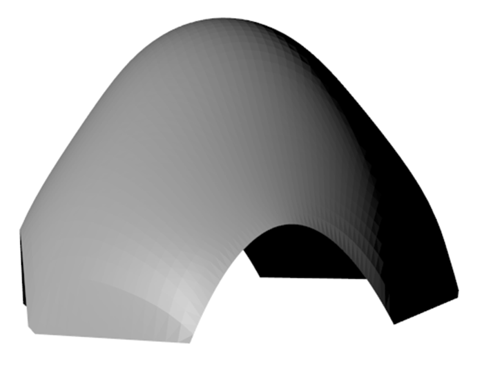
Fig. 16. Surface, built above the octagon.
6. Conclusion
In the present work, the problem of calculating and constructing a surface with the minimum possible area with a given edge and the volume of the region that this surface covers and other similar problems was considered. This variational problem is mathematically formulated and an algorithm for solving it is presented, which uses solutions of the equation of constant mean curvature for the case of surfaces given by the graph of a function and the gradient descent method for parametric surfaces of an arbitrary topological structure in the class of piecewise linear surfaces. The result is a module in the programming language Python, which is built into the Blender 3D modeling environment. This module allows you to interactively set the boundary conditions for solving the Plateau problem and set the topological type of the desired surface, and also perform the surface calculation and its visualization directly in the 3D view of the Blender program. The calculation result in the form of a polygonal surface can be saved as a 3D model in one of the standard file formats for vector 3D graphics.
In addition, the article describes the software implementation of the algorithm for calculating surfaces that minimize the functional of the mercy type in the class of surfaces defined by the function graph, and gives the figures of computed surfaces with different calculated regions and boundary conditions. The accuracy of the calculations averaged 0.01%.
The work is supported by a grant RFFI ? 15-41-02517.
References
[1]Klyachin A.A., Klyachin V.A., Grigorieva E.G., Visulization of calculation of minimal area surfaces. Scientific visualization. Electronic Journal . 2014,V .6, N 2, pp. 34-42.
[2] Klyachin A.A. On the uniform covergence of piecewise linear solutions of an equilibrium capillary surface equation. Journal of Applied and Industrial Mathematics, 2015, 9(3), pp. 381-391
[3] Douglas J. Solution of the problem of Plateau. Trans. Amer. Math. Soc. 33 (1931), p. 263-321.
[4] Radó T. On Plateau's problem. The Annals of Mathematics, Vol. 31, No. 3 p. 457–469.
[5] Klyachin A.A., Klyachin V.A., Grigorieva E.G. Visualization of stability and calculation of the shape of the capillary equilibrium surface. Scientific visualization. Electronic Journal . 2016, V.8, ?2. pp. 37-52.
[6] Vedenyapin A. D., Miklyukov V.M. Extrinsic dimensions of tubular minimal hypersurfaces. Math. USSR-Sb., V.59, ?1 (1988) , p.237-245.
[7] Miklyukov V. M., Tkachev V. G. Some properties of the tubular minimal surfaces of arbitrary codimension. Math. USSR-Sb, 68:1(1991), p.133-150 .
[8] Tkachev V. G. On the bore radius for minimal surfaces. Math. Notes, 59:6 (1996), p.657-660.
[9] Klyachin V. A. An estimation of spread for tubular minimal surfaces of arbitrary codimension. Sib. Math. J. V. 33. 1992. N. 5. p.~201–206.
[10] Mikhaylenko V.E., Kovalev S.N. Designing forms of modern architecture.Kiev Budivelnik, 1978. 138 .
[11] Abdyushev A.A., Miftahutdinov I.H., Osipov P.P.Design of shallow shells of minimal surface. News KSUAE, Building construction, building, 2009, N2 (12).
[12] Gatsunaev M. A., Klyachin A.A.On uniform convergence of piecewise linear solutions to minimal surface. Ufa Mathematical Journal. V. 6, N3 (2014), pp. 3-16.
[13] Klyachin A.A. Uniform triangulation of planar domains . Science Journal of VolSU. Mathematics. Phisics. 2011.N2(15).
[14] Serrin J. Gradient estimates for solutions of nonlinear elliptic differential equations. Acta Math., 1964, V.111, p. 247-302.
[15] Giaquinta M. On the Dirichlet problem for surfaces of prescribed mean curvature. Manuscripta Math., 1974, V.12, p. 73-86.
[16] Kapustina T.V. Minimal surfaces in Mathematica enviroment. International scientific-practical conference "Information Technologies in Education and Science-ITON 2014", IV International sciemtific seminar on mathematical modeling in systems of computer mathematics -"KAZCAS-2014"-conference materials and works of the seminar-Kazan. "Foliant", 2014.-P.216-219.
[17] Belchenko Yu. M., Shumun N.M. Simulation of 3-tissue for minimal surfaces. Ingenernyi Vestnik Dona. 2015. N 4-1, p.127.
[18] Kiselev A.V. Minimal surfaces associated with nonpolynomial contact symmetries. Fundamentalnaya i Prikladnaya Matematika, 2006, V. 12, N 7, p. 93-100.