IMPROVEMENT OF THE QUALITY OF RESTORING IMAGE WITH RADON INVERSE TRANSFORM
K.Ya. Kudryavtsev
National Research Nuclear University MEPhI (Moscow Engineering Physics Institute)
Contetns
2.2. Radon transform matrix value increasing algorithm.
Annex. MatLab 7.0 script for implementing the developed algorithm
Abstract
The creation of the image of internal contents of object without its physical corrupting applied in medicine, metallurgy and crystallography is based on X-ray radiation with the subsequent mathematical processing of received data. When the object is being scanned, the output ray intensity is equal to density distribution function along the ray path. Registration of emission calculated at different angles allows to obtain the original data used to reconstruct the image. Data used for image reconstruction has the form of matrix, each element of which is the result of integral evaluation along the determined line. The bigger matrix is, i.e. the more experimental data is available, the more exact image reconstruction will be possible. However, the number of experiments is often limited by medical, technical, economic and other reasons. As a mathematical tool for the reconstruction of the cross-sectional image of an object, a direct and inverse Radon transform is used. This paper proposes the algorithm of rising the quality of reconstructed image from Radon transform matrix by adding additional colums containing Radon transform in interjacent angle turn calculated with the help of developed approximation formulas. Doubling the number of Radon integral transformation matrix colums helps to significantly rise the quality of image being reconstructed with Radon inverse transformation.
Keywords: integral Radon transformation, Radon inverse transformation, image reconstruction
1. Introduction
The construction of the image of the internal contents of the object without its physical destruction, applied in medicine, metallurgy and crystallography is based on X-ray radiography, followed by mathematical processing of received data. The mathematical theory of image reconstruction is based on the direct and inverse integral Radon transformations [1-3]. The methodology of obtaining a two-dimensional laminogram includes two stages [4]. At the first stage, the projection data is formed, on the second stage - the image of the cross-section is reconstructed from the projection data. Modern computer tomographs mainly use systems with a fan-shaped or parallel beam. In the fan-shaped system, the rays diverge from the X-ray source in one subspace, but at different angles forming a fan. The radiation detectors are located on the arc on the other side of the studied object. In a parallel system (it will be analyzed hereinafter) a line-up of radiators is used, which forms parallel beams.
When the object is being scanned, the output intensity of the ray depends on the density of the studied object and is equal to the integral of the distribution function of the matter density along the ray trajectory. The registered radiation (Radon image or projection) measured for a set of parallel beams at different angles of rotation is represented as matrix R with the N × M dimension, each column of which corresponds to a certain rotation angle, and the number of lines is determined by the number of detector emitters. Actually, the reconstruction of the image is carried out using the inverse Radon transform operation (the inverse projection method [5]), the initial data for which are the values of the matrix R.
The larger the dimension of the matrix R is, i.e. the more detailed the studied object is scanned, the more accurate the image reconstruction will be. However, the high dimensionality of the R matrix is associated with a number of technical, medical and economic constraints. Therefore, it is desirable to have an algorithmic methodology for calculating the additional values of the matrix R on the basis of the available experimental data; that is where the issue of "missing data reconstruction” arises. In fact, the data is not missing. In order to improve the image recovery, it is desirable to increase the number of columns of the matrix R, thereby decreasing the discretization interval of the angle of rotation of the radiators line-up.
This paper [6] presents a comparison of various methodologies [7-13] for missing data recovery, such as:
· filling with the general average,
· filling with selection,
· filling by regression,
· spline interpolation methods,
· methodology of maximum likelihood filling,
· methods of factor analysis,
· methods of cluster analysis,
· algorithms of the family Zet (Wanga),
· methods of using neural networks.
The results of a comparative analysis [6] allow us to conclude that the best recovery results among all methods are shown by using the method of the missing value by spline interpolation by the present elements.
Consequently, in order to calculate the values of elements of additional columns of the matrix R, it is rational to use the approach based on the approximation methods.
This paper proposes an algorithm for improving the quality of image reconstruction by adding additional columns containing the Radon transform in the intermediate rotation angles calculated with the derived approximation formulas. The twofold increase in the number of columns of the matrix of the Radon integral transformation makes it possible to significantly improve the quality of image reconstruction with the inverse Radon transform.
2. Basic relation
The main idea of the proposed approach was previously presented by the author in paper [14]. Here we propose a more detailed and rigorous justification of mathematical relations.
Let us assume that there is Radon transform ![]() of
some image I. Normally Radon transform
of
some image I. Normally Radon transform ![]() is
shown as
is
shown as ![]() matrix.
matrix.
![]() –
is determined by image I size and line discretization interval τ along
which Radon integral transform.
–
is determined by image I size and line discretization interval τ along
which Radon integral transform.
![]() – is
determined by the number of angle rotation with
– is
determined by the number of angle rotation with ![]() step (within 0 - 180
angle degrees) of rotating coordinates, inside of which lines for evaluating
Radon transformation are drawn.
step (within 0 - 180
angle degrees) of rotating coordinates, inside of which lines for evaluating
Radon transformation are drawn.
Matrix element ![]() is
equal to the integral, evaluated along the line of perpedicular axis of
x-coordinate of rotating coordinate system and the beforementioned integral is
situated on a distance
is
equal to the integral, evaluated along the line of perpedicular axis of
x-coordinate of rotating coordinate system and the beforementioned integral is
situated on a distance ![]() from
the origin of coordinates. Angle rotation is equal to
from
the origin of coordinates. Angle rotation is equal to
![]() ,
,
where ![]() – is a turn step of moving coordinate
system. Line formula is evaluated with the following formula [1]
– is a turn step of moving coordinate
system. Line formula is evaluated with the following formula [1]
![]()
As shown in [5], according to Kotelnikov–Shannon formula in order to reconstruct the image in an acceptable quality the following correlation should be performed:
![]()
Hence increasing (doubling) of ![]() value
is of special interest, i.e. dicreasing of angle rotation step in the rotating
coordinate system.
value
is of special interest, i.e. dicreasing of angle rotation step in the rotating
coordinate system.
The simplest way to get ![]() R-matrix
is to add one column between each
R-matrix
is to add one column between each ![]() -matrix’s
columns and evaluate
-matrix’s
columns and evaluate ![]()
![]() elements
with line approximation formulas:
elements
with line approximation formulas:
![]()
![]()
![]()
However, as it will be shown below, the following
methodology will not result in quality rising of the reconstructed image, so
therefore it is required to develop a special algorithm, that will twice
increase ![]() value.
In other words, if
value.
In other words, if ![]() Radon
source transform of
Radon
source transform of ![]() dimention
is evaluated with
dimention
is evaluated with ![]() angle rotation step, that means the
algorithm should result in
angle rotation step, that means the
algorithm should result in ![]() Radon transform matrix of
Radon transform matrix of ![]() dimention,
that is to obtain a Radon transform evaluated with
dimention,
that is to obtain a Radon transform evaluated with ![]() angle
rotation step.
angle
rotation step.
2.1. Algorithm description
Let us analyze ![]() and
and ![]() coordinate
systems, whose center is connected with the center of the studied object and
rotated relative to each other by an
coordinate
systems, whose center is connected with the center of the studied object and
rotated relative to each other by an ![]() angle. (see Pic.1).
angle. (see Pic.1).
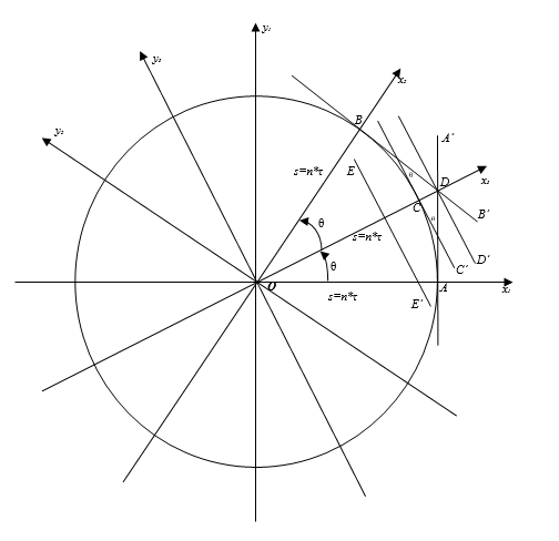
Pic.1 ![]() and
and ![]() coordinate
systems turned through
coordinate
systems turned through ![]() angle relative to each other.
angle relative to each other.
In ![]() coordinate
system the integral is being calculated along AA’ line
on s=nτ distance from the origin of the coordinates. In
coordinate
system the integral is being calculated along AA’ line
on s=nτ distance from the origin of the coordinates. In ![]() ,
coordinate system turned through
,
coordinate system turned through ![]() angle about
angle about ![]() , the
integral is evaluated along BB’ line also situated on s=nτ
distance from the origin of the coordinates. Let us analyze
, the
integral is evaluated along BB’ line also situated on s=nτ
distance from the origin of the coordinates. Let us analyze ![]() coordinate
system turned through
coordinate
system turned through ![]() angle
about
angle
about ![]() .
Please note that
.
Please note that ![]() coordinate
system is turned through
coordinate
system is turned through ![]() angle
about
angle
about ![]() .
.
It is required to estimate the value of the integral along CC’
line, which is perpendicular to ![]() axis
and which is situated on s=nτ distance from the origin of
the coordintes, i.e. to evaluate Radon transform with
axis
and which is situated on s=nτ distance from the origin of
the coordintes, i.e. to evaluate Radon transform with ![]() angle
rotation step two times smaller, that the original
angle
rotation step two times smaller, that the original ![]() .
.
Let us mark the integral value along AA’, BB’, CC’ lines with RAA’ ; RBB’ ; RCC’ accordingly. Integral RCC evaluation with formula
![]()
is incorrect, as CC’ line lies mostly out of BDA’ and ADB’ sectors. This averaging goes to RDD’ integral evaluation, i.e. to the integral along DD’ line, which goes between AA’ and BB’ lines and lies entirely within BDA’ and ADB’ sectors.
Hence let us assume that
![]()
The distance from the origin of the coordinates, where DD’ line lies is equal to
![]()
For the following transform let us introduce the following notation:
![]()
where ![]() .
First argument of
.
First argument of ![]() function
means the distance from the beginning of the coordinate origin, but the second
angle of rotation. So, for example,
function
means the distance from the beginning of the coordinate origin, but the second
angle of rotation. So, for example, ![]() means,
that the integral is evaluated along the line, which is perpendicular to
means,
that the integral is evaluated along the line, which is perpendicular to ![]() axis,
and rotated through the angle equal to zero, and is situated on
axis,
and rotated through the angle equal to zero, and is situated on ![]() distance from the
coordinate origin.
distance from the
coordinate origin.
For distance ![]() the
same formulas can be written, especially for EE’ line
the
same formulas can be written, especially for EE’ line
![]()
If values ![]() and
and ![]() are
evaluated, that means
are
evaluated, that means ![]() value
can be evaluated with the help of line approximation if CC’ line
is between EE’ and DD’ lines.
value
can be evaluated with the help of line approximation if CC’ line
is between EE’ and DD’ lines.
For that the following formula should be performed
![]()
or
![]()
If the inequaltion on the right is always performed, fot the inequation on the left the following can be written
![]()
or
![]()
Maximum value for ![]() is equal to
is equal to ![]() .
Hence
.
Hence
![]()
or
![]()
![]()
![]()
So the following restriction for ![]() angle rotation
connected to
angle rotation
connected to ![]() value
is obtained.
value
is obtained.
Assuming that the last ineqitation for ![]() angle rotation is
done, the following formula for
angle rotation is
done, the following formula for ![]() with
the help of line approximation is obtained
with
the help of line approximation is obtained
By simplifying the formula the result is

And taking into consideration, that
![]()
![]()
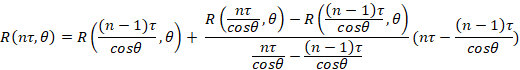
The final result will be
![]()
![]()
The obtained formula is rather interesting. There is a summand in it
![]()
which can be estimated as a simple line approximation like ![]() and
some correction
and
some correction
![]()
That estimates line position, along which there should be an integration with reference to lines used for evaluating approximation.
It should be mentioned that, if ![]()
![]()
i.e. the correction is not used, because CC’ direct line is entirely situated within BDA’ and ADB’ sectors and divides them into halves.
2.2. Radon transform matrix value increasing algorithm.
Given data: ![]() Radon
transform
Radon
transform ![]() matrix.
Angle rotation step is equal to
matrix.
Angle rotation step is equal to ![]() , i.e. integral calculation will be done
for the angles:
, i.e. integral calculation will be done
for the angles: ![]() ,
while
,
while ![]() .
.
Task: to evaluate R Radon transform ![]() matrix
with
matrix
with ![]() rotation angle step.
rotation angle step.
Let us divide the following algorithm into several stages.
Stage 1. Create ![]()
![]() -matrix
and fill it with zeros.
-matrix
and fill it with zeros.
Stage 2. Assign R-matrix odd columns to the
corresponding columns of ![]() -matrix.
-matrix.
![]()
Stage 3. Evaluate R-matrix even columns values for ![]() with the following
formulas:
with the following
formulas:
![]()
![]()
where ![]()
Stage 4. Evaluate ![]() column
value of R-matrix for
column
value of R-matrix for ![]() with the following formula:
with the following formula:
![]()
![]()
where ![]()
Stage 5. Evaluate R-matrix even columns values for
![]() with
the following formula:
with
the following formula:
![]()
![]()
where ![]()
Stage 6. Evaluate R-matrix ![]() column
value for
column
value for ![]() with the following formula:
with the following formula:
![]()
![]()
where ![]()
3. Estimation of efficiency
Estimation of efficiency of the proposed algorithm will be held in MatLab 7.0. 256 х 256 px phantom image is used fot the test. (see Pic. 2)
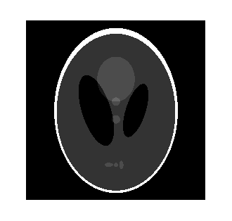
Pic. 2. Original phantom image
Let us choose angle rotation step as ![]() and
calculate Radon transform matrix with the help of radon
function in MatLab 7.0. As a result
and
calculate Radon transform matrix with the help of radon
function in MatLab 7.0. As a result ![]() .
. ![]() -matrix
is obtained. Here,
-matrix
is obtained. Here, ![]() .
.
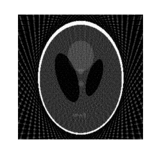
When performing Radon inverse transform with iradon function, the restored image is obtained (see Pic.3)
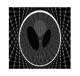
Pic. 3. Restored phantom image (angle rotation step ![]() )
)
As we can see the restored image quality is not very high,
as ![]() angle
rotation step is too large.
angle
rotation step is too large.
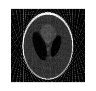
If angle rotation step is ![]() and
Radon transform
and
Radon transform ![]() matrix is evaluated and than Radon
inverse transform, the restored image has better quality. (see Pic.4)
matrix is evaluated and than Radon
inverse transform, the restored image has better quality. (see Pic.4)
Pic. 4. Restored phantom image (angle rotation step ![]() )
)
Choosing ![]() -matrix
as given source, let us make Radon transform for
-matrix
as given source, let us make Radon transform for ![]() R-matrix using the
abovementioned algorithm with formulas (1)-(5). Using Radon inverse transform,
the image like on Pic. 5 is obtained.
R-matrix using the
abovementioned algorithm with formulas (1)-(5). Using Radon inverse transform,
the image like on Pic. 5 is obtained.
Pic. 5. Phantom image restored from approximation matrix.
Comparing Pictures 3, 4 and 5 we can conclude, that the proposed algorithm improves the quality of the reconstructed image. Pic. 5 is visually less sharp than Pic. 4, but its quality is better, than that of Pic. 3.
In order to emphasize the significance of the proposed approximmation correction a Radon transform approximation matrix without correction should be built and than restored. (see Pic.6).
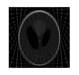
Pic. 6. Image restored from approximation matrix without approximation correction.
As it can be seen, ignoring the approximation correction do not lead to the increase of the image quality.
In addition to the subjunctive, visual estimation of the
proposed algorithm effectivity, the mean absolute deviation from exact values
of the evaluated approximation values should be found. As exact values, we take
Radon transform matrix of dimention ![]() with
an angle rotation step
with
an angle rotation step ![]() . The
estimation is calculated according to the following formula:
. The
estimation is calculated according to the following formula:
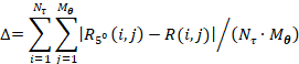
where ![]() –
Radom transform matrix elements with
–
Radom transform matrix elements with ![]() angle
rotation step.
angle
rotation step.
![]() – approximation transform matrix
elements, evaluated according to the previously discribed algorithm with
formulas (1)-(5).
– approximation transform matrix
elements, evaluated according to the previously discribed algorithm with
formulas (1)-(5).
The evaluation result is ![]() . To
put this in perspective, if approximation matrix is built without corrections,
the mean absolute deviation is
. To
put this in perspective, if approximation matrix is built without corrections,
the mean absolute deviation is ![]() .
According to Table 1 if lesser angle rotation steps are used (
.
According to Table 1 if lesser angle rotation steps are used (![]() )
) ![]() value
becomes even less.
value
becomes even less.
Table 1. Comparison of approximation matrix evaluation accuracy
|
|
|
|
|
|
|
11.2847 |
0.3261 |
34.6 |
|
|
11.2554 |
0.2969 |
37.9 |
|
|
11.1721 |
0.2138 |
52.25 |
|
|
11.1182 |
0.1598 |
69.57 |
|
|
11.0718 |
0.113 |
97.98 |
The proposed approximation correction significantly raises approximation quality, that is a substancial result.
The implementation of the described algorithm is presented in the application as a MatLab 7.0 script.
4. Conclusion
The following paper proposes an algorithm for raising the quality of the reconstructed image from Radon transform matrix by adding additional columns with Radon transform in the intermediate rotation angles, calculated from the derived approximation formulas.
The proposed algorithm consists of six stages:
- At the first stage: an R matrix with double number of columns is created and filled with zeroes;
- In the second stage: odd R-matrix columns are assigned to the corresponding columns of original matrix;
- At subsequent stages: the values of the elements of the matrix R are calculated from formulas (2) - (5).
Experimental validation showed, that the proposed algorithm allows to significantly improve the reconstructed image quality with the help of Radon inverse transform.
All the formulas obtained were experimentally checked in MatLab 7.0 system, which confirmed their full correctness.
References
1. Natterer F. The Mathematics of Computerized Tomography (Classics in Applied Mathematics, 32), Philadelphia, PA: Society for Industrial and Applied Mathematics, 2001 ISBN 0-89871-493-1
2. The Physics of Medical Imaging. Edited by Steve Webb Adam Hilger, Bristol and Philadelphia, 1991. ISBN 0-885274-367-0
3. Kudryavtsev K.Ya., Mikhaylov D.M. Radon integral transform on sparse rectangular grid. International Journal of Tomography and Simulation ISSN 2319-33362015, V. 28, N. 1, p. 89-104
4. Gruzman I.S., Kirichuk V.S., Kosyh V.P., Peretjagin G.I., Spektor A.A. Digital image processing in information systems: Textbook. NSTU, 2002. 352 p.
5. Kak A.C, Slaney M. Principles of computerized tomographic imaginng (Classics in Applied Mathematics, 33), Philadelphia, PA 19104-2688: Society for Industrial and Applied Mathematics, ISBN 0-89871-494-X
6. Abramenkova I.V., Kruglov V.V. Methods for recovering gaps in data sets. - Software products and systems, 2005, №2, p.18-22
7. Little R.J.A., Rubin D.B. Statistical analysis of data with omissions. - Moscow: Finance and Statistics, 1990.
8. Zagoruiko N.G. Applied methods of data and knowledge analysis. - Novosibirsk: Publishing house of the Institute of Mathematics, 1999.
9. Zagoruiko NG, Elkina VN, Timerkaev VS An algorithm for filling out blanks in empirical tables (Zet algorithm). Empirical prediction and pattern recognition. Novosibirsk, 1975. Issue. 61: Computing systems. p. 3-27.
10. Rossiev AA Modeling data using curves to restore gaps in tables. Methods of Neuroinformatics. Krasnoyarsk: KSTU, 1998.
11. Demidenko E.Z. Linear and nonlinear regression. Finance and Statistics, 1981.
12. Dvienko S.D. Non-hierarchical divisible clustering algorithm. Automation and telemechanics. 1999. № 4. P. 117-124.
13. Kruglov VV, Borisov VV Artificial neural networks. Theory and practice. M .: Hot line - Telecom, 2002.
14. Kudryavtsev K.Ya. Rising the Quality of Restor-ing Image with Radon Inverse Transform Basing on Spectral Approximation Formulas. International Journal of Tomography and Simulation ISSN 2319-3336 2016, V. 29, N. 2, p. 50-61.
Annex. MatLab 7.0 script for implementing the developed algorithm
P=phantom(256);
imshow(P);
dtheta=10;
theta1=0:dtheta:(180-dtheta);
[R1, xp] = radon(P, theta1);
theta2=0:dtheta/2:(180-dtheta/2);
[R2, xp] = radon(P, theta2);
I1=iradon(R1,dtheta);
I2=iradon(R2,dtheta/2);
Ntau=size(R1, 1);
NZero=(Ntau+1)/2;
Ntheta=size(R1, 2);
Ntheta2=2*Ntheta;
R1Appr = zeros(Ntau,Ntheta2);
R1ApprSimple = zeros(Ntau,Ntheta2);
Nel=size(R1Appr, 1) * size(R1Appr, 2);
Ktheta=(1-cos(pi*dtheta/360))/2;
for i=1:Ntheta
R1Appr(:,2*i-1)=R1(:,i);
end
for i=1:Ntheta
for n=1:NZero
j=NZero+n-1;
I0Nt=R1Appr(j,2*i-1);
I0Nt1=R1Appr(j-1,2*i-1);
if i < Ntheta
I2Nt=R1Appr(j,2*i+1);
I2Nt1=R1Appr(j-1,2*i+1);
else
I2Nt=R1Appr(j,1);
I2Nt1=R1Appr(j-1,1);
end
R1Appr(j,2*i)=(I0Nt+I2Nt)/2-(I0Nt-I0Nt1+I2Nt-I2Nt1)*(n-1)*Ktheta;
R1ApprSimple(j,2*i)=(I0Nt+I2Nt)/2;
end
end
for i=1:Ntheta
for n=1:NZero
j=NZero-n+1;
I0Nt=R1Appr(j,2*i-1);
I0Nt1=R1Appr(j+1,2*i-1);
if i < Ntheta
I2Nt=R1Appr(j,2*i+1);
I2Nt1=R1Appr(j+1,2*i+1);
else
I2Nt=R1Appr(j,1);
I2Nt1=R1Appr(j+1,1);
end
R1Appr(j,2*i)=(I0Nt+I2Nt)/2-(I0Nt-I0Nt1+I2Nt-I2Nt1)*(n-1)*Ktheta;
R1ApprSimple(j,2*i)=(I0Nt+I2Nt)/2;
end
end
Pogr=sum(sum(abs(R1Appr-R2)))/Nel
PogrSimple=sum(sum(abs(R1ApprSimple-R2)))/Nel
IAppr=iradon(R1Appr,dtheta/2);
IApprSimple=iradon(R1ApprSimple,dtheta/2);
figure,imshow(I1);
figure, imshow(I2);
figure, imshow(IAppr);
figure, imshow(IApprSimple);