CONCEPTION AND DEVELOPMENT EXPERIENCE OF "SINUS-D" SOFTWARE FOR RAPID VISUALIZATION OF DYNAMIC SYSTEMS SIMULATION
S.V. Ktitrov
National Research Nuclear University MEPhI (Moscow Engineering Physics Institute), Russian Federation
Contents
2. The choice of the class of the systems studied
3. Specifying equations and functions
4. Features of the implementation of system simulation
5. A graphical representation of simulation results
6. The portability and multiplatform
Abstract
The graphics subsystem is described in detail. It is designed to present the simulation results operatively. A lot of possibilities of graphic canvas include precise coordinate detection, the adjustment of the plot and the coordinate grid properties and others. Examples of its use for the visualization and comparative analysis of transient processes and phase portraits are presented.
The means implemented for the harmonic analysis of processes are presented. That helps to research the approximation quality by the partial sums of the Fourier series and the contribution of individual harmonics to the waveform shaping.
The conception of the software design includes its compactness and the possibility of using various software platforms. The software is single file compiled for Microsoft Windows, Apple OS X and Linux. It uses the common text file format for all platforms. Installation is not required.
The suggested approach to development of the similar programs is based on a combination of a built-in equation parser along with previously implemented set of typical nonlinear elements and intuitive interface.
Keywords: numerical solution, differential equations, difference equations, simulation, dynamic system, delayed system, nonlinear element
1. Introduction
Increasing requirements for the accuracy of the description of dynamic systems leads to the need to use nonlinear equations in their models, which, in turn, makes it more difficult, and more often, impossible to obtain an analytical description of the processes in the system under study. In this case, solving is performed by using numerical methods under different initial conditions, or modeling of the system. One of the most effective, fast and obvious ways of investigating a numerical solution is to analyze the graphical representation of either a particular solution, or family, including in the parametric form of a phase portrait.
Currently, there is a significant number of software tools that allow users to obtain a numerical solution of systems and display it in the form of graphs. Notable among these packages are Mathematica [1], Maple [2], Matlab/Simulink[3], their free counterparts Maxima[4], Octave[5], Freemat[6].
These software packages have a wide range of capabilities for numerical modeling, however their application raises the following difficulties:
· Due to the wide possibilities the size of the package is large and requires pre-installation on the computer;
· For the description of actions a special programming language is used, which, as a rule, increases flexibility, but requires study;
· The need to implement a number of non-linear elements (for example, backlash), and to turn explicitly to procedures makes the study less clear, bringing the procedure of describing and researching the system to the development of the simulation program in a high level language.
The article examines a specialized program "SINUS D" developed by the author. The program is intended for modeling nonlinear dynamic systems. Technical and design decisions taken during its creation are also presented. In its development, the goal was to obtain a compact software tool that provides a rapid numerical solution of complex nonlinear dynamical systems in a graphical form with maximum preservation of the visual presentation of both the original data and the results. This approach facilitates the use of the program by a student when performing laboratory work, as well as an engineer, a developer, a researcher, saving their time.
2. The choice of the class of the systems studied
The SINUS-D program was developed as a tool for research and initial design of complex automatic control systems. That determined the class of equations the solution of which is required to find.
The application of digital technology in control systems leads to the need to take into account the effects of signal quantization. Thus, the system should be considered as discrete-continuous. In general, the continuous non-linear automatic control system with concentrated parameters can be described by a system of ordinary differential equations (ODE) [7]:
 (1.1)
(1.1)
where ![]() – state
variables,
– state
variables, ![]() – output variables,
– output variables, ![]() – vector of input variables. In (1.1) it
is implied that all variables are related to one point in time
– vector of input variables. In (1.1) it
is implied that all variables are related to one point in time ![]() :
: ![]() ,
,
![]() ,
, ![]() .
The presence of a pure delay on one or more variables, that is, the use of
variables that depend on previous moments of time in equations leads to the
system of the form
.
The presence of a pure delay on one or more variables, that is, the use of
variables that depend on previous moments of time in equations leads to the
system of the form
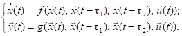 (1.2)
(1.2)
It should be noted that with the introduction of delayed variables (1.2) becomes a system of functional differential equations. It was decided to abandon the use of partial differential equations, since their solution requires the use of substantially different methods. On the other hand, a number of phenomena and processes usually described by equations with distributed parameters, can be approximately described by the system of the form (1.2) [8]. For example, the lag taken into account allows to simulate non-zero propagation time of the signal.
Difference equations are used to describe a discrete subsystem. Its representation in the state space has the form [9]:
![]() (1.3)
(1.3)
where ![]() is the number of the step corresponding to time
is the number of the step corresponding to time
![]() ,
,
![]() is
the sampling period of the system. The equations of the output in (1.1) - (1.3)
are algebraic equations, and, in contrast to differential and difference ones,
they do not assume the existence of initial conditions. Also, they are in
demand when you specify the subexpressions to simplify the form of the system.
is
the sampling period of the system. The equations of the output in (1.1) - (1.3)
are algebraic equations, and, in contrast to differential and difference ones,
they do not assume the existence of initial conditions. Also, they are in
demand when you specify the subexpressions to simplify the form of the system.
Any combination of types and number of equations are allowed in the model, but with algebraic equations in it only, it is possible to specify functional dependence. The frequency characteristics of the system can be a good example from the field of the automatic control theory. To construct them, operations on complex numbers are required. To avoid having the preparatory manual calculations (extraction of real and imaginary parts), the program has a special type of algebraic equations in which the operations on complex numbers are performed. The variable can also be defined as the solution of nonlinear algebraic equations, which provides the type of the equation "implicit function". Finally, to write duplicate expressions depending on a parameter, you can specify a functional expression as a function of one argument.
3. Specifying equations and functions
Commonly used matrix form of linear systems is convenient for the analytical description and analysis, but the definition of highly sparse matrix is tedious and not intuitive. In addition, this form requires the definition of the structure of the nonlinear part, which restricts the class of simulated systems. The program adopted the entry of the right side of equation "in line" in a natural mathematical form. Although it required developing a parser, but at the same time it made it possible not only to easily modify the right part, but also to change its structure easily by using nonlinear functions and products of state variables. Equations in the program are specified in a string in the form:
"variable" = "computed value of the right part"; "initial conditions",
moreover, additional descriptions of the variable is not required (Fig.1). To speed up input and to reduce the number of typos, you can use the Quick Input Panel, which contains a set of operations and functions, both built-in and user-defined (Fig. 2).
The user is able to use symbols of various alphabets, including Greek and Cyrillic for variable naming, that allows to set them in conventional notation and does not require renaming variables when they are set in the program.
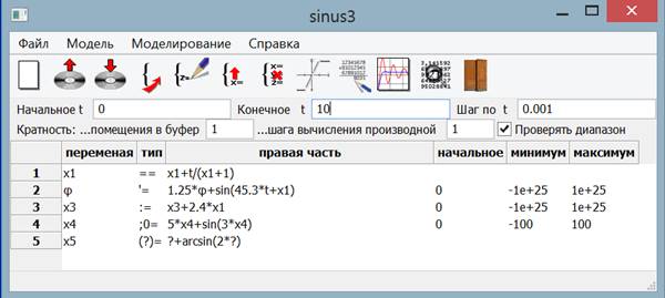
Fig. 1. Setting a system of equations, including equations of different types. The model includes: algebraic, differential, difference equation, implicit function and functional expression
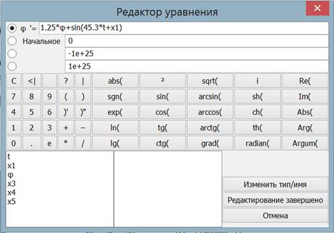
Fig. 2. The equation editor for the fast set of the right-hand side
To expand the class of non-linear systems studied, a wide set of typical nonlinear elements is implemented. These elements typically have one or more parameters. In order not to overload the right side of the equations, the user must assign a unique name to each nonlinearity with a certain set of parameters in use. For example, the set includes a piecewise linear function with discontinuities at the nodes. Let the function identifier, for example F2, be established as the set of nodes and the values of the function in them, including the left and right limits. Then the user can use the F2 name as a normal function without parameters: x1 + F2 (u) + ... Special elements are used to implement the so-called two-valued functions (the value of these functions depends on the sign of the first derivative of the argument), the function ranges that allow to generate an arbitrary piecewise-nonlinear function described in each area of individual expression, pseudorandom generators, etc. (Fig.3).
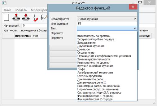
Fig.3. Setting functions with parameters
The described method of reference is used for elements such as delay, time quantizer and zero-order extrapolator, which allows one system to avoid restrictions imposed by a single sampling clock or a single delay.
4. Features of the implementation of system simulation
The investigation of the system dynamics involves obtaining
a description of the processes of the system in time, and the time is the same
for (1.1) and (1.3). To implement the model time, a dedicated variable
indicated by the symbol ![]() is provided. This variable is changed with a
constant step, called a simulation step. The use of solving methods with a
variable step was considered unnecessary, since the study of systems with
discontinuous right-hand side and discrete-continuous systems is planned.
is provided. This variable is changed with a
constant step, called a simulation step. The use of solving methods with a
variable step was considered unnecessary, since the study of systems with
discontinuous right-hand side and discrete-continuous systems is planned.
To solve the system of ordinary differential equations, we use the explicit fourth-order Runge-Kutta method [10]. To execute the method step, four calls to the right side of the system of differential equations are required. At the same time, in a complete simulated system, equations of other types may be present. Difference equations must be calculated once per one step, the algebraic ones may be used by the researcher as a means of computing the right-side subexpressions of differential or difference equations, or, on the contrary, as an output equation. Thus, the algebraic equations must be calculated after all the intermediate steps of the Runge-Kutta method. Let's consider how the program resolves this contradiction.
Algebraic equations (more precisely, expressions or formulas) are computed sequentially in the order they are defined. The value of the variable computed in the preceding expression is immediately available for use in subsequent expressions and right-hand sides of the differential equations. This is done to comply with the following principle (let's call it the substitution principle): if the right side of an algebraic expression substitutes for a variable determined by an expression, it does not change the result. To comply with this principle, the sequence of algebraic expressions must be formed without using variables on their right-hand sides, the algebraic expressions for which are described below. If this cannot be avoided, the value of the variable from the previous iteration is used.
The sequence order of differential equations is insignificant: moving to the next step is carried out simultaneously for all state variables, combined into the vector.
Let us consider the implementation of the substitution
principle by using variables specified by algebraic expressions on the
right-hand side of the differential equations. Algebraic expressions are calculated
each time before calculating the right-hand side of the differential equations.
On the other hand, expressions for output variables assume algebraic
transformations after the transition to the next step. To satisfy this
requirement, without violating the substitution principle, the program performs
the transition to the next step in time as follows: the values of
the right sides of the equations are calculated in the order shown in Table 1.
The digits indicate the order of calculation of expressions when one step of
integration is performed, ![]() is the simulation step. Algebraic expressions
are calculated using the values of the variable from differential
equations obtained as a result of the transition to the step k+1. The result of
this calculation can also be considered as preparing information for the
right-hand sides of the differential equations for the next step, which is
taken into account in the calculation scheme. To preserve the schema, algebraic
expressions are applied to the initial conditions before the first step.
is the simulation step. Algebraic expressions
are calculated using the values of the variable from differential
equations obtained as a result of the transition to the step k+1. The result of
this calculation can also be considered as preparing information for the
right-hand sides of the differential equations for the next step, which is
taken into account in the calculation scheme. To preserve the schema, algebraic
expressions are applied to the initial conditions before the first step.
Table 1. The order of computations of algebraic and differential equations in the performing of the k-th step of the Runge-Kutta method
|
The value of the model time |
Algebraic equations |
Differential Equations |
|
|
8 (k-1step) |
1 |
|
|
2 |
3 |
|
|
4 |
5 |
|
|
6 |
7 |
|
|
8 |
1 (k+1 step) |
For the correct simulation of a discrete-continuous system, it is necessary that the sampling clock be substantially larger than the modeling step, but at the same time it is a multiple of it. This means that the transition to the next value determined by the difference equations must be made substantially less frequently than for differential equations. To realize the possibility of modeling systems containing simultaneously several quantizers in time with different sampling cycles, it is proposed to use an element of the "extrapolator" type, giving the right part of the equation to its input. This element evaluates its argument only at the time points corresponding to the next step.
The transition from ![]() to
to ![]() is accompanied by a
check on the output of a variable from the allowable range. The minimum and
maximum values for each variable can be specified not only by a number, but
also by an algebraic expression involving other variables of the system. When
the variable leaves the specified range, the simulation stops. This feature of
the program allows you to simulate systems by the piecewise method and to
simulate systems with a variable structure.
is accompanied by a
check on the output of a variable from the allowable range. The minimum and
maximum values for each variable can be specified not only by a number, but
also by an algebraic expression involving other variables of the system. When
the variable leaves the specified range, the simulation stops. This feature of
the program allows you to simulate systems by the piecewise method and to
simulate systems with a variable structure.
The values of all the computed variables and their corresponding model time are stored in the internal array. If the dimension of the system is large enough, and the simulation step is small, the size of the buffer memory may be insufficient. A small step is usually used to ensure the stability of the numerical method, but the display of results is planned with a larger step, so, using the "memory multiplicity" parameter, you can store the values of the variables by skipping part of the steps. The same principle governs the step of calculating the derivatives of expressions that can be computed by a simple difference in the right parts of the equations.
The equations of the type "implicit function" at each time step are solved by the method of Golden section, which minimizes the residual error. The initial condition is taken either by the initial condition, which is set by the user along with the range of admissible values, or its value at the previous iteration.
The user can enter the right parts of the equations either in a text string form or he can generate it using the Quick Entry Panel, as discussed in section 3. Before the simulation starts, the equations are syntactically analyzed, a tree-like structure of objects (elementary operations and functions connected in accordance with the given expression) is formed. For example, to compute the right part of the differential equations of the form
x3’=1/T1*(F(u+x1+x2)-x3),
where u, T1 are variables of algebraic equations, F is user-defined nonlinearity, the structure the structure will be built in form shown in Fig. 4.
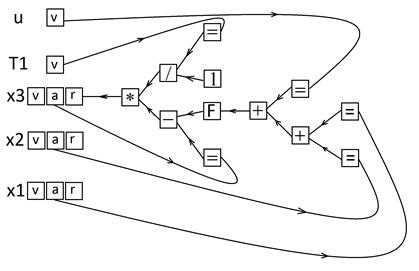
Fig. 4. The right part of the differential equations calculation
Expressions are evaluated recursively through the constructed tree, causing the elementary operations via function pointers. Each operation specified in the rectangle corresponds to the function call. The symbol "=" indicates the operation of copying the value. Three types of cells are used to store the values for each variable corresponding to the differential equation. Type "v" corresponds to the calculated value at the k-th step. It is the simulation result. The cell of type "a" stores the right-hand argument that is used to calculate the intermediate steps in the Runge-Kutta method. Type "r" intended to store the value of the right part in the intermediate step. The separation of the cells of types "a" and "r" provides the use of values of the vector of state variables corresponding to one time. F denotes the nonlinearity specified by the user. Along with the function type, a set of parameters is stored. This set is associated with the given identifier used to calculate the value. Building a tree in memory allows you to assume that the program performs a preliminary compilation of the code. This compilation is implemented by means of the high-level language without using the features of the target computer architecture. The comparison of the speed of the SINUS-D program and the code compiled with optimization shows a lag of only 2-5 times, depending on the expressions on the right part of equations. Note that the simulation software monitors exceptions, such as division by zero, the function arguments outside its domain, the value of a variable out of the specified range.
The user can view the obtained numerical results in the form of a table and, if necessary, write it to a file (Fig. 5).
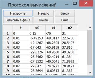
Fig. 5. The view showing numerical simulation results
5. A graphical representation of simulation results
The most effective way to analyze the results of numerical simulation of dynamic systems is the graphical representation of the results. The following display capabilities are implemented:
- multi-window mode, which allows to represent data in different coordinate systems;
- Ability to display several graphs in one coordinate system (Fig. 6);
- the possibility of enlarging the fragments of the plots;
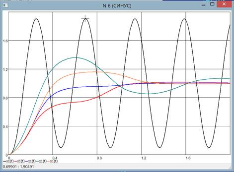
Fig. 6. The display of multiple graphs when you select corrective devices in the suppression of self-oscillations. The cursor coordinates allows to determine the amplitude of self-oscillations
- determination of exact values of coordinates under the cursor (Fig. 6);
- color coding of graphs and coordinate axes;
- automatic detection of the display range;
- automatic determination of the division value of the grid for obtaining round values;
- use of the shift of the grid divisions for more convenient marking of divisions;
- saving images in various raster (bmp, jpg, png, tiff) and vector formats (ps, svg);
- deleting plots, moving them between windows;
- change the thickness of the lines for drawing the graphs.
The capability to save the graph to a file in the form of a text value table and to load it from a file is implemented. The accepted format allows you to load dependencies, including those generated in other programs and to use "SINUS-D" as a graph viewer. For this, there are options that suppress the output of the main window for specifying the model - only the window with the graph is displayed on the screen.
The program provides the opportunity to plot the dependence of the random variable computed from any other variable (Fig. 7), which allows to draw separate phase trajectories (Fig.8). Taking into account the possibility to combine multiple graphs in the same coordinate systems, it is possible to draw phase portraits as well (Fig.9).
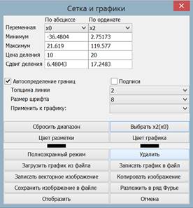
Fig. 7. Dialog description of the properties of the graph
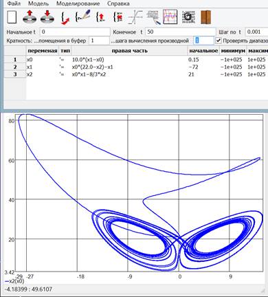
Fig. 8. The phase trajectory is a strange Lorenz attractor
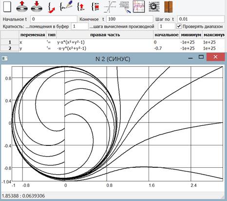
Fig.9. The phase portrait of a limit cycle in a nonlinear system
As we can see in Fig. 7, the means for frequency analysis of the obtained process are provided. The user can decompose the obtained dependence into a Fourier series using a given number of harmonics, and then superimpose the partial sum of the series on the graph. The maximum number of harmonics available for decomposition is limited by the Nyquist-Shannon theorem, and the decomposition interval is automatically calculated on the basis of the frequency function, but can be set manually by the user. Fig. 10 illustrates the Gibbs phenomenon using 1, 3, 5, 7 and 25 harmonics. The harmonic parameters are represented in the amplitude / phase format. The user can change an arbitrary parameter, plot such a function, can estimate the contribution of particular harmonics in the signal.
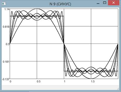
Fig. 10. The demonstration of the Gibbs phenomenon
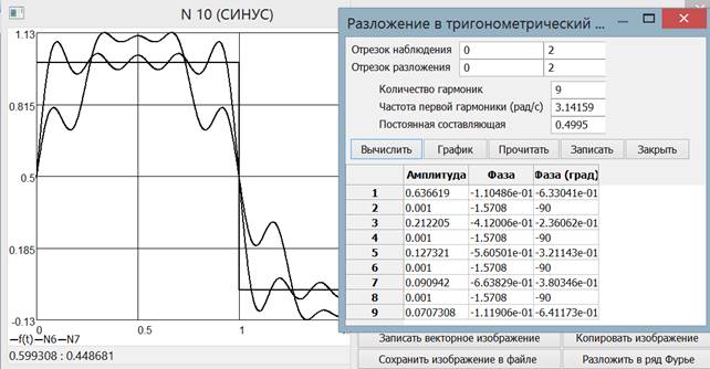
Fig. 11. The comparison of the Fourier series expansion up to the 9th harmonic with the expansion, in which there are no 3 and 5 harmonics
6. The portability and multiplatform
The GUI has been developed using wxWidgets library, which provides graphics toolkit for major operating systems: Microsoft Windows, Apple OS X and Linux. The program is made monolithic by using static linking of the required libraries, so it does not require special installation procedures to migrate to another computer. Copying to another computer is sufficient. Its size is about 1 MB due to the tool for dynamic compression of the executable file. Files of the program have unified format and use UTF-8 encoding. Compact size, multiplatform, ready-to-use conception allow you to constantly have the program on the portable medium as a tool for operational simulation and visualization of processes.
7. Conclusion
The "SINUS D" software for modeling of nonlinear dynamic systems provides wide opportunities for graphical analysis of processes in such systems. The program is oriented primarily to simulate discrete-continuous systems of automatic control and can serve as a graphical tool for constructing complex nonlinear functions, including complex-valued ones, and even means of solving systems of nonlinear algebraic equations.
The developed program is extremely compact, requires no installation and can be used as readily available means to solve complex problems. To start working with the program, no special training or learning of programming languages is required, which is confirmed by many years of experience as the basis for a laboratory workshop.
During the development of the program, a number of tasks concerning the design of both the computing core and the construction of a graphical interface were solved. The experience of creating this program can be used in the future when developing other programs for the rapid visualization of the results of numerical experiments.
References
5. www.gnu.org/software/octave
7. Zadeh L, Desoer Ch. Linear System Theory. The State Space Approach. McGraw-Hill New York. 1970.
8. J. Hale. Theory of Functional Differential Equations. Springer-Verlag. NewYork Heidelberg Berlin. 1977.
9. Kuo B. Digital Control Systems. Holt, Rinehart and Winston Inc.1980.
10. Butcher J.C. Numerical Methods for Ordinary Differential Equations. John Wiley&Sons,Ltd, 2003.