THE EVOLUTION OF THE PLASMA FORMATION IN THE GAS MEDIUM, MODELING WITH VISUALIZATION OF THE GRID NODES DYNAMICS AND THE INTERACTION OF SHOCK AND THERMAL WAVES
P.V.Breslavskiy1, O.N.Koroleva1,2, A.V.Mazhukin1,2
1M.V. Keldysh Institute of Applied Mathematics, RAS, Moscow, Russia
2National Research Nuclear University MEPhI (Moscow Engineering Physics Institute), Moscow, Russia
e-mail: vim@modhef.ru
Contents
2. Mathematical statement of the problem
3. Arbitrary nonstationary system of coordinates
4. Finite difference approximation
5. Choice of the adaptation function
Abstract
The structure of the shock and thermal waves in the air in the expansion of the plasma is investigated. Simulations have shown that the characteristics of plasma formation, the occurrence of shock and heat waves are dependent on a number of influence parameters and environment properties. The nature of the interaction of thermal and hydrodynamic flow quality varies with the magnitude of the thermal conductivity of the medium. High thermal conductivity leads to thermal waves of two different types - subsonic and supersonic. The structure of the solutions of supersonic mode is represented as two consecutive waves - thermal and hydrodynamic. The subsonic structure of the solution presented in the form of three waves: the isothermal shock wave located between the two (subsonic and supersonic) thermal waves. To solve nonlinear equations of hydrodynamics with a thermal conductivity we use finite-difference approach, combined with the procedure of dynamic adaptation of the computational grid that allows us to explicitly locate the strong (shock waves) and weak (thermal wave front) discontinuities. Visualization and analysis of the results of calculations on a grid containing 30 nodes are carried out in comparison with self-similar solutions found for similar problems. The work was financially supported by the Russian science Foundation (project code 15-11-00032).
Keywords: laser plasma processes, fluid dynamics, dynamic grid adaptation method, nonlinear heat conduction, visualization.
1. Introduction
Significant progress in the computer industry, concerning both technical and software components, couldn’t but affect the scope of such a scientific activity, as convenience and clarity of display of the research work results. The Internet technology extension and the emergence of electronic publications not only reduce the time of analysis but also (thanks to visualization) improve the perception of the represented results. All of the above applies not only to multi-dimensional problems, but even in one-dimensional statements it is possible to visualize the dynamics of the considered processes.
The class of problems describing real physical processes taking place, and having at the same time exact or similar solutions, is rather narrow [1-5] and, often, their implementation requires a substantial simplification of the original statement. However, despite this, they continue to remain relevant [6]. The development of new computational algorithms and the validity of the numerical solutions of complex nonlinear systems, especially in areas such as gas and fluid dynamics [7-10], laser treatment [11-14], and plasma physics [15-17], rely significantly on self-similar solutions of simplified model problems [6].
Numerous applications of pulsed laser treatment (pulsed laser ablation (PLA) [18-20], pulsed laser deposition (PLD) [21], the production of nanomaterials [22-24]) make it an attractive destination for fundamental research. Many previous experimental and theoretical investigations have been focused on the study of the adiabatic expansion of laser plasma in a vacuum, although most applications of PLA performed in the presence of ambient gas [25, 26]. The presence of a gas environment dramatically changes mode laser effect on the target, modifies the conditions for the emergence of laser plasma and complicates the description of the process of laser ablation due to changes in the structure of the plasma torch, the characteristics of the expanding plasma and the occurrence of radiation and shock waves [27-29].
The basic mechanisms of energy transfer in the problems of gas dynamics, describing the expansion of completely ionized plasma, along with radiation, are convective and conductive mechanisms. Accordingly, mathematical models for these problems are underlain by the radiation transfer equations and the fluid dynamic equations with nonlinear heat conduction. Much attention to the influence of nonlinear heat conduction on the interaction between thermal and hydrodynamic processes was given in [6, 30]. It was established that problems of this class have widely different solutions, and self-similar solutions were obtained in a relatively narrow range of parameters. The nature of the interaction of thermal and hydrodynamic fluxes changes qualitatively with varying heat conduction of the medium. Purely hydrodynamic phenomena such as shock waves dominate at low heat conduction. The high thermal conductivity of the medium leads to supersonic and subsonic thermal waves interacting with shock waves.
Computationally, the fluid dynamic equations with nonlinear heat conduction represent a complicated problem to solve. A typical solution to such problems has a complex structure and includes strong discontinuities (shock wave fronts), weak discontinuities (thermal wave fronts), and regions of steep temperature, pressure, density, and velocity gradients. The presence of discontinuous solutions, steep-gradient regions, and their fast propagation in space impose strict requirements on the efficiency of the computational algorithms used, primarily, on the grid generation principles rather than on the quality of the difference schemes applied [31, 32].
The nonlinear fluid dynamic equations with heat conduction are solved using finite-difference schemes combined with dynamic adaptation. The basis used finite-difference schemes are based on the principles of conservation [33] and monotonicity [34]. The construction principles for finite-difference algorithms with dynamic adaptation as applied to a wide class of parabolic and hyperbolic equations with moving and fixed boundaries were described in detail in [35-38] (see also the references therein on adaptation methods).
The main goal of this paper is to study the dynamics of plasma formation and interaction between a shock and thermal waves in a gaseous medium. Another of the objectives is to develop efficient computational algorithm to control the distribution of grid nodes and the ability to explicitly trace the strong and weak discontinuities as applied to fluid dynamics problems with nonlinear heat conduction. Generally, the use of dynamic adaptation [35-38] reduces the total number of nodes on several orders of magnitude compared to grids of fixed nodes. Visualization and analysis of the numerical results obtained on a 30-node grid with dynamic allocation of nodes are implemented in comparison with self-similar solutions found earlier [38, 39].
2. Mathematical statement of the problem
In the Eulerian formalism, the problem of the expansion of laser plasma with a nonlinear thermal conductivity is described by the complete system of equations of gas dynamics with heat conduction
|
|
(2.1) |
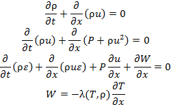
with the equations of state
![]()
Here, ρ is the density, u is the velocity, P is the pressure, ε is the internal energy, T is the temperature, R is the gas constant, γ is the adiabatic index, W is heat flux, and λ is the thermal conductivity. It is assumed that λ is a power function of the temperature and density: λ(T, ρ)= λ0 T a ρb.
Initial conditions. At t = 0, it is assumed that the background velocity is zero and the background temperature and density are a constant:
|
|
(2.2) |
Boundary conditions. They are formulated taking into
account the fact that strong and weak discontinuities are explicitly tracked in
the dynamic adaptation method. The left plane ![]() , when
, when
![]() , is a
source of motion and heat. For this reason, two boundary conditions determining
the velocity of the piston and the heat flux are specified on the piston
surface:
, is a
source of motion and heat. For this reason, two boundary conditions determining
the velocity of the piston and the heat flux are specified on the piston
surface:
|
|
(2.3) |
The particular values of a, b, and n are matched with a self-similar solution and will be specified later.
The background values are preserved on the right boundary ![]() :
:
|
|
(2.4) |
Relations on the shock front. Since the temperature
across the front shock ![]() is
continuous, we write three conservation laws (Rankine–Hugoniot relations):
is
continuous, we write three conservation laws (Rankine–Hugoniot relations):
|
|
(2.5) |
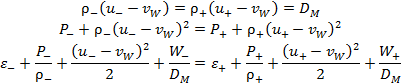
Here, the minus and plus indices denote the variables on different sides of the shock wave, ʋW is the velocity of the shock wave, and DM is the mass flux across the shock front.
3. Arbitrary nonstationary system of coordinates
According to the dynamic adaptation method (see [35]), we proceed to an arbitrary non-stationary coordinate system. In the new variables (q, τ), system (2.1) becomes
|
|
(3.1) |
|
|
(3.2) |
|
|
(3.3) |
|
|
(3.4) |
where ψ is the Jacobian of the inverse transformation and Q is the adaptation function to be determined.
Since all the perturbations arise on the left boundary (![]() ) and
propagate rightward, the unperturbed domain is excluded from consideration in
order to reduce the computational costs. For this purpose, the right boundary
is shifted toward the left one to be a small distance away from it. When a
perturbation arises on the right boundary, it is treated as a free surface
) and
propagate rightward, the unperturbed domain is excluded from consideration in
order to reduce the computational costs. For this purpose, the right boundary
is shifted toward the left one to be a small distance away from it. When a
perturbation arises on the right boundary, it is treated as a free surface ![]() propagating
at the velocity of thermal or gas-dynamic perturbations. The new boundary
propagating
at the velocity of thermal or gas-dynamic perturbations. The new boundary ![]() coincides
with a temperature wave front, which is a weak discontinuity whose propagation
velocity ʋT
is determined by a relation derived from the equation of motion in the moving
coordinate system. The other conditions are transferred from (2.4) without change:
coincides
with a temperature wave front, which is a weak discontinuity whose propagation
velocity ʋT
is determined by a relation derived from the equation of motion in the moving
coordinate system. The other conditions are transferred from (2.4) without change:
|
|
|
|
Thus, on proceeding to an arbitrary non-stationary coordinate system, the original differential model (2.1) is transformed into extended model (3.1)–(3.4), which has been supplemented by the inverse transformation equation (3.4). Accordingly, the necessary additions are introduced in initial (2.2) and boundary (2.3)–(2.4) conditions:
|
|
|
(3.5) |
|
|
|
(3.6) |
|
|
|
(3.7) |
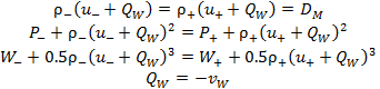
In the non-stationary coordinate system, discontinuities are explicitly introduced in the solution and, after a shock wave appears, system (3.1)–(3.4) is solved in two subdomains divided by the shock front. At the front, the resulting solutions are matched using the Rankine–Hugoniot conditions:
|
|
|
(3.8) |
4. Finite difference approximation
System (3.1)–(3.8) was numerically solved on the grid
|
|
The differential equations were approximated by finite differences on staggered grids. Specifically, we used the following family of difference schemes, in which the density ρi+1/2, the temperature Ti+1/2, the pressure Pi+1/2, and the internal energy εi+1/2 were determined at the half-integer points, while the velocity ui and the function Qi were determined at the integer points:
|
|
(4.1) |
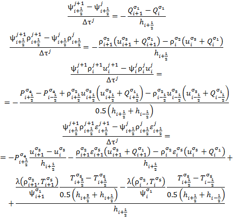
Here, ![]() , а σr = σ1, σ2, … are the weighting factors
determining the degree to which the difference scheme is implicit. If σ1 = σ2 =…= 0, we obtain a
completely explicit difference scheme with an O(Δτ
+ h2) approximation error. If σ1 = σ2 =…= 1, the scheme is
completely implicit with the same order of accuracy. In the case of σ1 = σ2 =…= 0.5, we have a scheme
with an O(Δτ2 + h2)
approximation error. The computations were performed using the completely
implicit difference scheme with O(Δτ + h2)
accuracy.
, а σr = σ1, σ2, … are the weighting factors
determining the degree to which the difference scheme is implicit. If σ1 = σ2 =…= 0, we obtain a
completely explicit difference scheme with an O(Δτ
+ h2) approximation error. If σ1 = σ2 =…= 1, the scheme is
completely implicit with the same order of accuracy. In the case of σ1 = σ2 =…= 0.5, we have a scheme
with an O(Δτ2 + h2)
approximation error. The computations were performed using the completely
implicit difference scheme with O(Δτ + h2)
accuracy.
For the functions {u, Q } = ƒ specified
at the integer points of w,
their values at the half-integer points were determined by the formula ![]() .
Similarly, the values of the functions {ψ, ρ, T, P,
ε} = ƒ at the integer points were
determined in terms of their values at the half-integer points:
.
Similarly, the values of the functions {ψ, ρ, T, P,
ε} = ƒ at the integer points were
determined in terms of their values at the half-integer points: ![]() . The
flowchart of the calculation algorithm is shown in Fig.1. The algorithm
involves two internal iteration blocks based on Newton’s method. The first
block solves the difference analogue of the energy equation, while the second
block solves the analogues of the continuity equation, the equation of motion,
and grid point redistribution equation (the first three equations in (4.1)).
Both blocks are included in the external iteration cycle. If the number of
external iteration steps exceeds fifteen or the number of internal iteration
steps exceeds twenty, the time step is decreased by 10%. If the number of
external iteration steps is less than four, the next time step is increased by
1%. The initial value for each unknown grid function is specified as
. The
flowchart of the calculation algorithm is shown in Fig.1. The algorithm
involves two internal iteration blocks based on Newton’s method. The first
block solves the difference analogue of the energy equation, while the second
block solves the analogues of the continuity equation, the equation of motion,
and grid point redistribution equation (the first three equations in (4.1)).
Both blocks are included in the external iteration cycle. If the number of
external iteration steps exceeds fifteen or the number of internal iteration
steps exceeds twenty, the time step is decreased by 10%. If the number of
external iteration steps is less than four, the next time step is increased by
1%. The initial value for each unknown grid function is specified as ![]() .
.
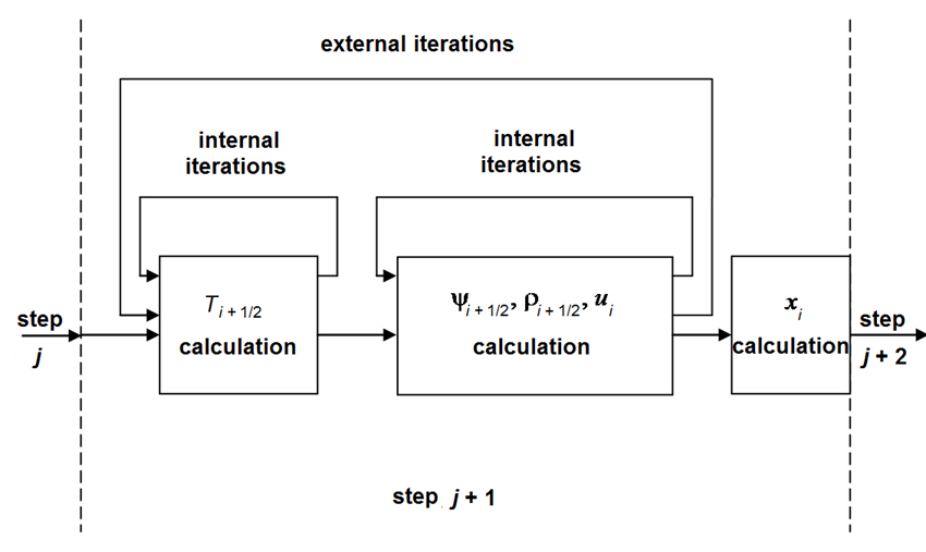
Fig.1. The flowchart of the calculation algorithm.
The Rankine–Hugoniot relations (3.8) are required to hold on
the shock wave ![]() .
Since the equations involve six unknowns, three of them are determined by
solving system (3.1)–(3.4) at the boundary points. These are the density ρ– and
the velocity u– ahead
of the shock front and the velocity u+ behind the shock front. The remaining three unknowns
(the shock propagation velocity ʋW, the density ρ+ behind the shock front, and
the temperature T– =
T+ on the
shock front) are determined by relations (3.8).
.
Since the equations involve six unknowns, three of them are determined by
solving system (3.1)–(3.4) at the boundary points. These are the density ρ– and
the velocity u– ahead
of the shock front and the velocity u+ behind the shock front. The remaining three unknowns
(the shock propagation velocity ʋW, the density ρ+ behind the shock front, and
the temperature T– =
T+ on the
shock front) are determined by relations (3.8).
5. Choice of the adaptation function
The grid point distribution in the dynamic adaptation method is controlled using the adaptation function Q. In the case of steep-gradient solutions, this function is usually determined from the quasi-stationarity principle (see [35–38]), according to which we choose a non-stationary coordinate system in which all the physical processes proceed as steady-state ones and the corresponding time derivatives are relatively small. Setting the time derivatives in the equations equal to zero yields the sought adaptation function.
The general solution to the complete system of fluid dynamics equations (3.1)–(3.4) is determined by the sum of the velocity, density, and temperature. These functions have different (frequently oppositely directed) spatiotemporal distributions. A controllable grid point distribution for the system of equations must take into account the features of the spatiotemporal distributions for all the solution components.
In the general case, the adaptation function in fluid dynamics problems can be determined using the entire system of equations [36-38]. In this paper, the function Q is found from energy equation (3.3), whose solution depends on the velocity, density, and heat conduction. In nonconservative form, the energy equation is
|
|
|
Based on the quasi-stationarity principle, we set ![]() to
obtain the equation
to
obtain the equation
|
|
(5.1) |
By taking into account the particular form of the equations
of state ![]() and
differentiating the heat flux
and
differentiating the heat flux ![]() , the
function Q is determined by simple rearrangements in Eq. (5.1):
, the
function Q is determined by simple rearrangements in Eq. (5.1):
|
|
(5.2) |
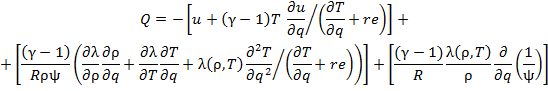
where re is a regularizing constant that is a lower bound for the derivative as it tends to zero.
After the difference approximation, the first square bracket in (5.2) exerts a contraction effect on the grid points in u and T. The second square bracket takes into account the influence of nonlinear heat conduction and exerts a contraction effect with respect to ρ and T. The last term is of the diffusion type. If λ(ρ, T ) ≠ 0, it has a smoothing effect and, in particular, prevents the intersection of grid point trajectories.
The features of the class of problems under consideration are determined by two factors. The first is that the thermal conductivity is a power function of the temperature. At low temperatures (near zero), since the thermal conductivity is low, the dissipating effect of the diffusion term decreases sharply and may become insufficient for an optimal grid point distribution. The second factor is that the original problem is represented in the form of a free-surface problem. The original domain may then increase by many orders of magnitude. Accordingly, the values of ψ increase as well, which also strongly reduces the diffusion component. To eliminate these effects, it is reasonable to supplement Q with a function obtained from the diffusion approximation [21] taking into account the presence of moving boundaries:
|
|
|
where D is the diffusivity. Its value is determined by the geometric size of a cell (the mesh size h), by the velocity of the boundary points (ʋl, ʋr), and by the minimum of the function (ψmin) over the entire domain:
|
|
|
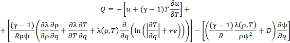
Additionally, it is reasonable to represent the ratio of two temperature derivatives in Eq. (5.2) in the form of the derivative of a slowly varying logarithmic function:
|
|
|
In view of the features described above, the adaptation function can be finally written as
|
|
(5.3) |
6. Simulation results
The problem of a piston accelerating in a medium with nonlinear heat conduction was simulated by solving system (3.1)–(3.4) with initial conditions (3.5), boundary conditions (3.6) and (3.7), Rankine–Hugoniot relations (3.8), and adaptation function (5.3). Since the solution was compared with self-similar profiles, the problem was solved with the constants corresponding to the self-similar solution [38]:
|
|
|
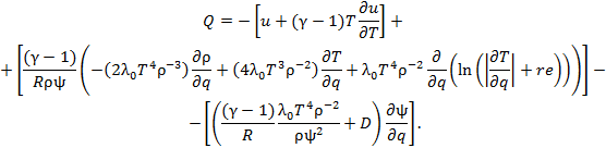
In view of the temperature dependence of the thermal conductivity and the density λ(T, ρ) = λ0 T 4 ρ-2, the adaptation function given by (5.3) became
|
|
(6.1) |
The total number N of nodes (the position of which in all the figures mentioned markers) in all the computations is 30.
The constants λ0 multiplying the thermal conductivity corresponded to the nondimensional thermal conductivities in the self-similar solutions. Dimensionless constant λₒ = 1 corresponds to a value of 6.18·10-24 m7/(kg·s3·K5) . The following are the values of the dimensionless constants λₒ, corresponding to a certain self-similar mode.
One purpose of this study is to compare the characteristics of the developing plasma flow depending on the degree of nonlinearity of the thermal processes. The simulation showed that the nature of the interaction of thermal and hydrodynamic flow quality varies with the magnitude of the thermal conductivity of the medium. The high thermal conductivity of the medium gives rise to thermal waves which are caused by the form of the hydrodynamic motion is divided into two different types - the supersonic and subsonic. The supersonic heat propagates with finite speed of the initial background. Behind the front of the supersonic thermal wave appears isothermal shock wave. Temperature wave propagating at subsonic speeds, is going for the shock wave in front of it, and are characterized by vanishing heat flux W, maximum density ρ and the local minimum of the temperature T. A change in the heat transfer regime depends on the degree of nonlinearity of heat conduction and is determined by the value of λ0. At value λ0 less than λ* (λ0 < λ*) (for the considered modes λ* ≈ 30) subsonic propagation of heat is formed, and supersonic one is formed if λ0 ≥ λ*. We consider one subsonic thermal wave with λ0 = 10 (Fig. 2), and two with λ0 = 50 and λ0 = 200 (Fig. 3, 4) corresponding to supersonic propagation of heat.
Subsonic propagation of heat. Thermal wave with λ0 = 10 is characterized by subsonic heat transfer. After the shock wave generation subdomain between left boundary and shock wave involved 22 meshes and subdomain between the shock wave and the outer boundary contained 8 meshes. Figure 2 shows the evolution of temperature, density, velocity and the Jacobian of the inverse transformation from the beginning of the calculation t = 0 to the end t = 1 ms. The curves with dashed line depict the self-similar solution, and solid line with markers shows the numerical solution (markers correspond to computational grid nodes). The Jacobian of the inverse transformation characterizes the spatial step change compared to its initial value. At the time of the shock wave generation numerical results have nothing to do with self-similar one. However, there is a significant change in the parameters of the plasma flow after the formation of the shock wave. A subsonic thermal wave is appeared. Isothermal shock wave approaches the external temperature supersonic wave. There are sharp changes in the solution in these areas, resulting in a restructuring of the computational grid. The maximum concentration of nodes is achieved at the fronts of thermal waves. The numerical solution is gradually approaching the self-similar one. At t = 0.01 ms numerical solution coincides with self-similar one very close. At the end t = 1 ms numerical solution agrees with self-similar one, and their spatial profiles are identical, Figure 2.
Fig. 2. Simulation results for λₒ= 10 (solid line with markers – numerical solution, dashed line - self-similar solution).
The structure of the solutions in the subsonic mode (Figure 2) is represented in the form of three waves following each other (from right to left):
· supersonic thermal wave generated by the shock wave;
· a shock wave, which is isothermal jump with continuous temperature and discontinuous density and velocity;
· subsonic thermal wave coming after the shock.
At the front of the supersonic thermal wave (weak discontinuity) the x-derivatives of all the functions are discontinuities, while all the physical quantities are continuous, as occurs in the case of one nonlinear heat equation without allowance for fluid dynamics. Moreover, the heat flux, velocity, density, and temperature increase sharply behind the front.
Shockwave (isothermal discontinuity) is characterized by a strong change of all sizes.
Another area of abrupt change of physical quantities is a subsonic thermal wave front. It is characterized by maximum density, zero heat flow and the local minimum temperature.
Dimension of computational domain and spatial grid steps in the physical space are characterized by the function ψ (x, t), which shows how many times the mesh size and the domain as a whole change at every instant of time. Since the domain had moving boundaries such that the right one (the front of the supersonic wave temperature) moved much faster than the left one (front of the plasma), (i.e., ʋT >> ʋp), the function ψ(x, t) suggests that the geometric size of the perturbed physical region was increased in excess of 10 orders of magnitude over the indicated time interval. The local minima of ψ(x, t) correspond to areas with the highest gradients of the solution and coincide with subsonic and supersonic thermal waves Figure 2.
Supersonic propagation of heat. Supersonic thermal wave is characterized by supersonic heat transfer, which predetermines a weak interaction between thermal and hydrodynamic processes. Nevertheless, when the thermal conductivity depends strongly on the temperature and the rate of heat transfer is high, the supersonic mode can become dominant in heat transfer.
Fig. 3. Simulation results for λₒ= 50 (solid line with markers – numerical solution, dashed line - self-similar solution).
Figures 3 and 4 display the spatial profiles of the gas dynamic functions, temperature, and ψ for λₒ = 50 and 200, respectively. We use a grid with the total number of nodes N = 30, the distribution of which is noted by markers.
The structure of the supersonic propagation of heat solution is much simpler than that of the solution in the subsonic mode. It consists of two waves (thermal and hydrodynamic) following one another. Their velocities of propagation are different, and the front of the supersonic thermal wave is much ahead of the shock front (see Figs. 3, 4). The front positions correspond to a weak and a strong discontinuity, respectively, near which the mesh is the densest.
For λₒ = 50 (see Fig. 3), the velocity of thermal wave is comparable to the velocity of the shock wave, and the region of supersonic heating is much smaller than for a medium with high heat conduction (λₒ = 200) (see Fig. 3), for which the thermal wave velocity is much higher. Spatial profiles of gas dynamic functions and temperature in this case (λₒ = 50) are different from both the subsonic mode (λₒ = 10) and the mode with λₒ = 200 when the thermal wave velocity is differed substantially from the velocity of the shock wave. The temperature and density have no extrema typical for subsonic heat propagation, but due to the proximity of the velocities of the thermal and shock waves in the mode with λₒ = 50 thermal and hydrodynamic components of the plasma flow interact interacts with each other, which leads to a significant decline in the density and temperature gradients approaching the shock wave front.
In all the modes Fig. 2-4 the numerical results (solid line with markers) are compared with the earlier obtained self-similar solutions for the piston problem (dashed line) [38]. At t = 0.01 ms numerical solution coincides with self-similar one very close. At the end t = 1 ms numerical solution agrees with self-similar one, and their spatial profiles are identical, which indicates the reliability and quality of the results. The highest temperature is reached in the left boundary at the end of calculation t = 1 ms and, as one would expect, is greater at a lower thermal conductivity. For λₒ = 10 - Tmax ≈ 3 keV, while for λₒ = 200 - Tmax ≈ 1.9 keV.
Fig. 4. Simulation results for λₒ= 200 (solid line with markers – numerical solution, dashed line - self-similar solution).
Features of dynamic adaptation. From a point of view of dynamically adapted grid generation, a brief analysis both supersonic and subsonic modes (see Figs. 2–4) reveals the following features. Both regimes are characterized by three moving boundaries: the left boundary with the known law of motion (2.3), the shock wave front (strong discontinuity), and the front of a supersonic temperature wave (weak discontinuity) propagating against a temperature background. The laws of motion for the last two are unknown and are determined in the course of the solution. All the three moving boundaries are explicitly tracked in the solution.
Since the left boundary and the supersonic thermal wave front are explicitly tracked, the trivial-solution regions can be excluded from consideration. This is especially important in non-stationary problems, such as wave propagation in which a perturbation originates near one of the boundaries and propagates toward the other. At long times, a perturbation can sweep a region that differs from the original one by several orders of magnitude. In such situations, the exclusion of unperturbed regions from consideration plays an important role and allows one to construct economic computational algorithms.
An explicit track of the shock front helps overcome the difficulties associated with discontinuous solutions.
In addition to the moving boundaries, the problem of thermal wave propagation involves several regions of rapid variations in all the solution functions: the temperature, density, and velocity. There are two such regions in the supersonic mode and three in the subsonic.
Thus, dynamic adaptation must take into account the behavior of all the functions (temperature, velocity, and density) and the presence of moving boundaries. All these conditions are satisfied by the adaptation function Q (6.1).
7. Conclusions
Simulations have shown that the dynamic characteristics of the plasma substantially related to the degree of nonlinearity of the thermal processes. The major features of the solution to the fluid dynamic equations with nonlinear heat conduction include the presence of three moving boundaries and two (supersonic) or three (subsonic) regions of rapid variations in all the solution functions. All the moving boundaries were explicitly tracked. For two of them (namely, for the shock front and the temperature wave front), the law of motion was not known beforehand and was determined in the course of the solution.
The considered problem of plasma expansion showed the effectiveness and applicability of the dynamic adaptation method proposed for solution. For this class of problems, an adaptation function was proposed that controls the grid point distribution depending on the features of the solution. The adaptation function has a complex structure and consists of several terms. Some of them are determined by the diffusion approximation and take into account the variations in the size of the computational domain caused by the motion of the front of a plasma torch and by propagation of weak and strong discontinuities. The other terms are determined by the quasi-stationarity principle and are responsible for mesh refinement in regions with steep gradients of temperature, density, and velocity.
The dynamic adaptation method makes it possible to use grids with extremely few nodes. In all the computations, the total number of nodes was N = 30, although the computational domain was increased in excess of 10 orders of magnitude.
The use of visualization tools allows display visibly the complex dynamics of interconnected physical processes and determined their controlled distribution of nodes of computational grids with dynamic adaptation.
Acknowledgments
This work was financially supported by the Russian science Foundation (project code 15-11-00032).
References
1. Boudesocque-Dubois C., Lombard V., Gauthier S., Clarisse J. An adaptive multidomain Chebyshev method for nonlinear eigenvalue problems: Application to self-similar solutions of gas dynamics equations with nonlinear heat conduction. JCP, 2013, vol. 235, pp. 723-741.
2. Clark D., Tabak M. A self-similar isochoric implosion for fast ignition. Nucl. Fusion, 2007, vol.47, pp. 1147–1156.
3. Murakami M., Sakaiya T., Sanz J. Self-similar ablative flow of nonstationary accelerating foil due to nonlinear heat conduction. Phys. Plasmas, 2007, vol. 14, pp. 269-292.
4. Toque N. Self-similar implosion of a continuous stratified medium. Shock Waves, 2001, vol.11, pp. 157–165.
5. Poljanin A.D., Vjaz'min A.V. Tochnye reshenija dvumernyh i trehmernyh nelinejnyh uravnenij teplo- i massoperenosa [Exact solutions of two-dimensional and three-dimensional nonlinear equations of heat and mass transfer]. Reports of the Academy of Sciences, 2003, vol. 390, № 2, pp. 214-218. [in Russian]
6. Volosevich P.P., Levanov E.I. Avtomodel'nye reshenija zadach gazovoj dinamiki i teploperenosa [Self-similar solutions of gas dynamics and heat transfer]. Publishing house MIPT, 1997. [in Russian]
7. Poljanin A.D., Zajcev V.F., Zhurov A.I. Metody reshenija nelinejnyh uravnenij matematicheskoj fiziki i mehaniki [Methods for solving nonlinear equations of mathematical physics and mechanics]. Fizmatlit, 2005, 256 p. [in Russian]
8. Samarskij A.A., Popov Ju.P. Raznostnye metody reshenija zadach gazovoj dinamiki [Difference methods for solving of gas dynamics]. Nauka, 1992. [in Russian]
9. Tannehill J.C., Anderson D.A., Pletcher R.H. Series in Computational and Physical Processes in Mechanics and Thermal Sciences, Taylor & Francis, 1997.
10. Popov I.V., Frjazinov I.V. Metod adaptivnoj iskusstvennoj vjazkosti chislennogo reshenija uravnenij gazovoj dinamiki [The method of adaptive artificial viscosity numerical solution of the equations of gas dynamics]. KRASAND, 2014, 288 p. [in Russian]
11. Gladush G.G., Smurov I. Physics of Laser Materials Processing. Theory and Experiment. Springer, 2010, 390 p.
12. Mazhukin V.I. Kinetics and Dynamics of Phase Transformations, in: Metals Under Action of Ultra-Short High-Power Laser Pulses. Ch. 8, pp.219 -276. in: Laser Pulses – Theory, Technology, and Applications”, Ed. by I. Peshko. 2012, p. 544, InTech, Croatia.
13. Lasers in Materials Science. Editors: M. Castillejo, P. M. Ossi, L. Zhigilei. Springer Series in Materials Science, vol. 191, 387 p., Springer, 2014
14. Mazhukin V.I., Mazhukin A.V., Lobok M.G. Comparison of Nano- and Femtosecond Laser Ablation of Aluminium. Laser Physics, 2009, vol. 19, № 5, pp. 1169 - 1178.
15. Morel V., Bultel A., Cheron B.G. Modeling of thermal and chemical non-equilibrium in a laser-induced aluminum plasma by means of a Collisional-Radiative model. Spectrochimica Acta Part B, 2010, vol. 65, pp.830–841.
16. Sy-Bor Wen, Mao X., Liu C., Greif R., Russo R. Expansion and radiative cooling of the laser induced plasma. Journal of Physics: Conference Series 59, 2007, pp. 343–347.
17. Mazhukin V.I., Smurov I., Flamant G. Simulation of Laser Plasma Dynamics: Influence of Ambient Pressure and Intensity of Laser Radiation. J. Comp. Phys., 1994, vol.112, no. 20, pp. 78-90.
18. Synthesis and Photonics of Nanoscale Materials IX. Editors: F. Trager, J. J. Dubowski, D.B. Geohegan. Proceedings of SPIE, 0277-786X, vol. 8245, SPIE, Bellingham, WA, 2012.
19. Lee J.Y., Ko S.H., Farson D.F., Yoo Ch.D. Mechanism of keyhole formation and stability in stationary laser welding. J. Phys. D: Appl. Phys. 2002, vol. 35, pp.1570–1576.
20. Laser-Surface Interactions for New Materials Production. Editors: A.Miotello, P.M.Ossi. Springer Series in Material Science vol.130, 358 pp. Springer, 2010.
21. Chrisey D.B., Hubler G.K. Pulsed Laser Deposition of Thin Films. John Wiley & Sons, New York, 1994.
22. Al-Shboul K.F., Harilal S.S., Hassanein A. Spatio-temporal mapping of ablated species in ultrafast laser-produced graphite plasmas. Appl. Phys. Lett. 2012, vol. 100, 221106, pp. 1-4.
23. Menendez A.-Manjon, Barcikowski S., Shafeev G.A., Mazhukin V.I., Chichkov B.N. Influence of beam intensity profile on the aerodynamic particle size distributions generated by femtosecond laser ablation. Laser and Particle Beams, 2010, vol. 28, pp. 45–52.
24. Sintez nanorazmernyh materialov pri vozdejstvii moshhnyh potokov jenergii na veshhestvo [The synthesis of nanoscale materials under the influence of powerful energy flows on the matter]. The Russian Academy of Sciences. Siberian Branch. Institute of Thermal named after S.S.Kutateladze, Novosibirsk, 2009, 461 p. [in Russian]
25. Panchatsharam S., Bo Tan, Venkatakrishnan K. Femtosecond laser-induced shockwave formation on ablated silicon surface. J. Appl. Phys., 2009, vol. 105, 093103.
26. Harilal S.S., Miloshevsky G.V., Diwakar P.K., LaHaye N.L., Hassanein A. Experimental and computational study of complex shockwave dynamics in laser ablation plumes in argon atmosphere. Physics of Plasmas, 2012, vol. 9, 083504, pp. 1-11.
27. Mazhukin V.I., Uglov A.A., Chetverushkin B.N. Low-temperature laser plasma near metal surfaces in the high-pressure gases. A Review. Kvantovaya elektronika, 1983, vol. 10, no. 4, 679-701.
28. Mazhukin V., Smurov I., Flamant G. Simulation of Laser Plasma Dynamics: Influence of Ambient Pressure and Intensity of Laser Radiation. J. Comp. Phys., 1994, vol. 112, no. 20, pp. 78-90.
29. Harilal S.S., Brumfield B.E., Phillips M.C. Lifecycle of laser-produced air sparks. Physics of Plasmas, vol.22, pp. 063301(1-13) (2015).
30. Marshak R . An influence of the radiation on the behavior of the shock waves. Phys. Fluids, 1958, no. 1, pp. 24 -29.
31. Liseikin V.D. Grid Generation Methods. Second Edition. Springer, 2010, pp.390.
32. Gil'manov A.N. Metody adaptivnyh setok v zadachah gazovoj dinamiki [Methods of adaptive grids in gas dynamic problems]. Fizmatlit, 2000, 248 p. [in Russian]
33. Samarskij A.A. Teorija raznostnyh shem [The theory of difference schemes]. Nauka, 1989, 616 p. [in Russian]
34. Samarskii A.A., Mazhukin V.I., Matus P.P., Mozolevskii I.E. Monotone Difference Scheme for Equations with Mixed Derivatives. Computers & Mathematics with Application, 2002, vol. 44, pp. 501 - 510.
35. Mazhukin V.I., Demin M.M., Shapranov A.V., Smurov I. The method of construction dynamically adapting grids for problems of unstable laminar combustion. Numerical Heat Transfer, Part B: Fundamentals, 2003, vol.44, N 4, pp. 387 – 415.
36. Breslavskiу P.V., Mazhukin V.I. Dinamicheski adaptirujushhiesja setki dlja vzaimodejstvujushhih razryvnyh reshenij [Dynamically adapted grids for interacting discontinuous solutions]. Computational Mathematics and Mathematical Physics, 2007, vol. 45, no. 4, pp. 717 - 737. [in Russian]
37. Mazhukin A.V., Mazhukin V.I. Dinamicheskaja adaptacija v parabolicheskih uravnenijah [Dynamic adaptation to parabolic equations]. Computational Mathematics and Mathematical Physics, 2007, vol. 47, no. 11, pp. 1911 - 2034. [in Russian]
38. Breslavskiy P.V., Mazhukin V.I. Metod dinamicheskoj adaptacii v zadachah gazovoj dinamiki s nelinejnoj teploprovodnost'ju [Method for dynamic adaptation in problems of gas dynamics with nonlinear thermal conductivity]. Computational Mathematics and Mathematical Physics, 2008, vol. 48, no. 11, pp. 2067 - 2080. [in Russian]
39. Breslavskiy P.V., Koroleva O.N., Mazhukin A.V. Simulation of the dynamics of plasma expansion, the formation and interaction of shock and heat waves in the gas at the nanosecond laser irradiation. Mathematica Montisnigri, 2015, Vol XXXIII, pp. 5-24