OPTICAL TOMOGRAPHY OF REFRACTING OBJECTS WITH OPAQUE REGIONS
Afanasyev V.V., Ignatenko A.V., Voloboy A.G.
Keldysh Institute of Applied Math RAS
Graphics and Media Lab CMC MSU
vafanasjev@graphics.cs.msu.ru, ignatenko@graphics.cs.msu.ru, voloboy@gin.keldysh.ru
Contents
3. Data and specific of optical tomography
4. Limitations of classic model
4.1 Problem of complete attenuation
5.1 Absorption data extraction
Abstract
Classic computed tomography techniques like ART are widely used for reconstruction of objects scanned in X-ray devices, where almost every object can be made transparent by increasing radiation power and its absorption can be measured with some accuracy. But the classic model cannot be applied to reconstruction of objects which absorption is so high that it does not transmit any radiation: such cases are possible in X-ray tomography with a low-power radiation source and also are frequent in optical tomography.
The article explains difficulties faced by classic ART algorithms in optical tomography in case of opaque regions presence in the scanned object. The ART method modification is proposed for this case.
Keywords: computed tomography, optical tomography, ART.
1. Introduction
With the advent of physically-based photorealistic rendering, computer graphics application area extended considerably. The created algorithms and software became useful in architecture, urban development, lighting systems designing, in car and aircraft industry and other areas. Preliminary lighting calculations and realistic rendering of virtual model improve the efficiency of production process substantially.
An interesting problem is using realistic images in diamonds processing and gems cutting. The rendered images allow improving the process of making technical products and jewelry on different stages of processing: from rough stones scanning till cutting. The most difficult thing in this problem is high material transparency. Visualization of projected cuts requires using correct algorithms of light distribution modelling and also high precision of cut geometry. Primary geometry of inclusions in rough stone is determined using computed tomography methods.
Computed tomography is a problem of internal object structure reconstruction using a set of its projections. The most spread type of computed tomography is X-ray computed tomography. A review of X-ray tomography is made in article [1]. X-ray tomography as one of non-destructive scanning methods is used in medicine for disease diagnostics, for animals research [2][3], for defect detection in machine parts, in geologic research [4] and other areas/
X-ray tomography scanner consists of emitter, sensor and holder for object between them. The emitter irradiates X-rays with fixed intensity, radiation is absorbed inside the object and then sensor detects residual rays’ intensity. During object rotation on some trajectory a set of projections is got and internal object structure is reconstructed using these projections.
Different ray beam configurations are possible depending on emitter type: flat/volumetric, parallel/divergent beams. Depending on emitter type one can use flat or volumetric tomography algorithms.
Radiation absorption in the material obeys Beer’s law:
![]() (1)
(1)
Where ![]() is measured intensity on the sensor,
is measured intensity on the sensor, ![]() is
emitter intensity irradiated in this direction,
is
emitter intensity irradiated in this direction, ![]() is
absorption index distribution along the ray.
is
absorption index distribution along the ray.
The exponent index in (1) contains definite integral on ![]() segment. If we change
it to improper integral on
segment. If we change
it to improper integral on ![]() interval
and consider all lines intersecting the observable region, we get Radon
transform.
interval
and consider all lines intersecting the observable region, we get Radon
transform.
For clearness, we will consider 2-dimensional absorption distributions on figures.
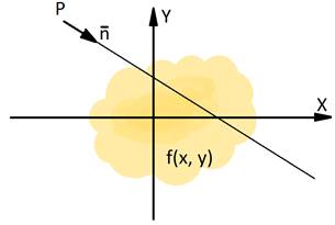
Fig. 1. Radon transform for one line
Radon transform of function is a function ![]() which
is defined for every line in space
which
is defined for every line in space ![]() , every value of this function is an
improper integral of function
, every value of this function is an
improper integral of function ![]() along the corresponding line. The fig. 1
shows this for 2-d function
along the corresponding line. The fig. 1
shows this for 2-d function ![]() . Function
argument is represented in vector form.
. Function
argument is represented in vector form.
![]() (2)
(2)
It is supposed that improper integrals converge, so, the
function ![]() is limited and is close to 0 on the
infinity. In practice only functions defined in some limited areas are
considered. Also the function should be limited and infinite absorption in some
part of area is illegal.
is limited and is close to 0 on the
infinity. In practice only functions defined in some limited areas are
considered. Also the function should be limited and infinite absorption in some
part of area is illegal.
We can represent the Radon transform as a function of direction
and line displacement from coordinates center as it is shown on fig. 2. We get
a 2-d function ![]() where
where
![]() –
is line displacement and
–
is line displacement and ![]() is angle between line and X axis. This
function is called sinogram for parallel projection. In practice, the function
is angle between line and X axis. This
function is called sinogram for parallel projection. In practice, the function ![]() is examined in limited
area, this leads to finite area of sinogram definition.
is examined in limited
area, this leads to finite area of sinogram definition.
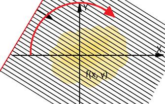
Fig. 2. Radon transform
Under certain restrictions on function ![]() and
sensor trajectory the inverse Radon transform exists. [5] However, if
there is a noise and other inaccuracy in input data, it is unstable. Also
inverse Radon transform is computationally expensive.
and
sensor trajectory the inverse Radon transform exists. [5] However, if
there is a noise and other inaccuracy in input data, it is unstable. Also
inverse Radon transform is computationally expensive.
2. Existing approaches
Volume reconstruction from projections methods are divided into direct and iterative. [6] Direct methods include convolution and back projection, Fourier synthesis methods. Classic iterative method is ART (algebraic reconstruction technique).
The main idea of ART algorithms is minimization of
difference between the unknown function ![]() and
its real value by iterative approximation of observable projection on every
single image. Many implementations of this idea exist, including additive,
multiplicative and other ART methods. [7]
and
its real value by iterative approximation of observable projection on every
single image. Many implementations of this idea exist, including additive,
multiplicative and other ART methods. [7]
Additive ART is the simplest method. Algorithm input is
sinogram (a discrete set of projections, in 2-d case there are ![]() projections with
projections with ![]() values in each) and
geometric characteristics of projections (rays direction and sensor physical
size). The output should be the desired function
values in each) and
geometric characteristics of projections (rays direction and sensor physical
size). The output should be the desired function ![]() ,
defined on a net of size
,
defined on a net of size ![]() . The function is considered to be
piecewise, i.e. it has constant value inside one net cell.
. The function is considered to be
piecewise, i.e. it has constant value inside one net cell.
Firstly, the net is initialized with some values (for example, 0). Then, the following steps are carried out iteratively some previously set number of times or until matching some condition:
Next projection value selection from pixel ![]() of projection
of projection ![]() . The way of its
selection can be determined by special order of projections and pixels bypass,
the simplest method is sequential selection.
. The way of its
selection can be determined by special order of projections and pixels bypass,
the simplest method is sequential selection.
Generating line corresponding to current projection value. Line parameters are calculated from known projection geometry.
Calculation of integral ![]() of
current function along the line.
of
current function along the line.
Counting signed difference ![]() between
known observed value of projection and current value of integral.
between
known observed value of projection and current value of integral.
Net traversal and correction of current function values along the line. Function correction in single cell is realized in the following way:
![]() (3)
(3)
Where ![]() is
regularization coefficient,
is
regularization coefficient, ![]() is the length of line segment inside
current cell,
is the length of line segment inside
current cell, ![]() is full length of line and net
intersection.
is full length of line and net
intersection.
Fig. 3 shows a schematic image of this process:
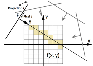
Fig. 3. Projections and pixels application
3. Data and specific of optical tomography
For clearness, here and below we will consider only refracting objects with flat faces. Scanning object through curved refracting surface cause additional distortion due to cameras’ optical system properties: sharpness and blur areas. Compensations of these effects do not refer directly to tomography algorithms and it will not be examined here.
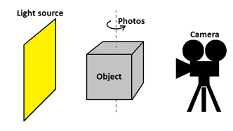
Fig. 4. Optical tomography scanner scheme
Optical tomography is similar to classic tomography, as it is shown on figure 4, but there is difference:
The light source is some luminous area with nonuniform light distribution. This distribution can be obtained from photo of the light source without the scanned object.
Every projection value is not a value of integral of function, it is a value of residual light intensity taking into account attenuation due to material absorption and surface transmission according to Fresnel equations. Also light reflection from all surfaces makes its contribution.
It is possible to get zero intensity value on projection that corresponds to infinite absorption. The infinite absorption is concordantly represented with zero projection values on all photos in corresponding areas. In classic model the integral of absorption index along the ray is taken and in the linear model no set of finite projection values exist that would represent the infinite value of absorption in some area of the volume. Analogic effect is possible in X-ray tomography, caused with some metal object when scanning with low radiation power.
Generally, the rays from one photo that were parallel in the air, after refraction on the surface can cross the target volume from more than one direction.
Rays density inside refracting object is variable and depends on incident angle before refraction.
Tomography data is discrete initially. All other values are also discrete for storage in memory and computations.
Quantization of rotation angle of the object relatively to sensor. There is a finite number of projections. Usually, a sample of projections with constant step is used.
Quantization of ray displacement from coordinates center. The sensor always has a finite number of pixels.
Quantization of residual radiation intensity.
Quantization of arguments of desired function ![]() . The function is
defined on a net with constant step.
. The function is
defined on a net with constant step.
Quantization of function ![]() values.
values.
Unlike X-ray tomography, in optical tomography it is possible that only a limited range of view angles is available during the scanning. It happens because of light refraction. For example, in case of scanning cube made of diamond (refracting index 2.4) moving around the cube, the internal volume can be observed from only about one half of directions. Fig. 5 shows the view directions inside the air when watching through one facet and also all observing directions of some point inside refracting material. There are 4 groups of directions inside the material with gaps between them.
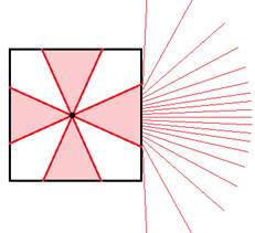
Fig. 5. Available directions inside the refracting cube
4. Limitations of classic model
Working with optical tomography data containing opaque regions, several disadvantages of linear model and classic methods were found:
4.1 Problem of complete attenuation
A complete attenuation of some area is impossible to handle
in linear model, because the sensor pixel gives zero intensity that corresponds
to infinite value of absorption index integral along the ray. The infinite
value can be replaced with some big constant ![]() . But this will mean
that whatever the actual form of opaque region may be, the integral along any
ray intersecting it will be equal to
. But this will mean
that whatever the actual form of opaque region may be, the integral along any
ray intersecting it will be equal to ![]() not
depending on intersection length. An internal inconsistency of absorption index
integrals appears between the rays going from different directions. A
distribution of absorption index inside the region that would cause such
measured values of all integrals generally does not exist. Fig. 6 shows an
example of such area: two rays going from different directions have
intersection length with it equal to
not
depending on intersection length. An internal inconsistency of absorption index
integrals appears between the rays going from different directions. A
distribution of absorption index inside the region that would cause such
measured values of all integrals generally does not exist. Fig. 6 shows an
example of such area: two rays going from different directions have
intersection length with it equal to ![]() and
and ![]() respectively.
respectively.
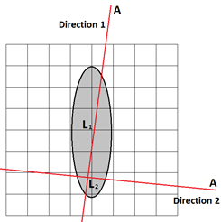
Fig. 6. Intersection of long opaque region
On each iteration of tomography algorithm a new projection is applied on which the intersection length between rays and the area can be greater or smaller than on the previous projection. So, the correction will be positive or negative. Even in the case of precise input data the oscillations of absorption inside this area will be continuous. The group of directions from which the rays have smaller length of intersection with area will increase the absorption and otherwise, the group of directions with greater intersection length will decrease the absorption in the same area.
A method for decreasing artefacts caused by complete attenuation in X-ray tomography based on maximum likelihood method is described in article [8]. In the present article a simpler approach is proposed that is discussed using the example of optical tomography.
4.2 Discretization problem
The discrete nature of input data causes another problem. Let the completely opaque region has sharp border. It can be different from the net voxels borders. “Rasterization” of this area’s contour can be different on voxels when observing them from different directions and in this case the oscillations of absorption index along the entire ray can happen from iteration to iteration. This effect is possible not only because of inaccuracy in input data, but also on absolutely accurate input data (synthetic) because of difference between discretization frequency of voxel net and sensor that will certainly occur on different directions.
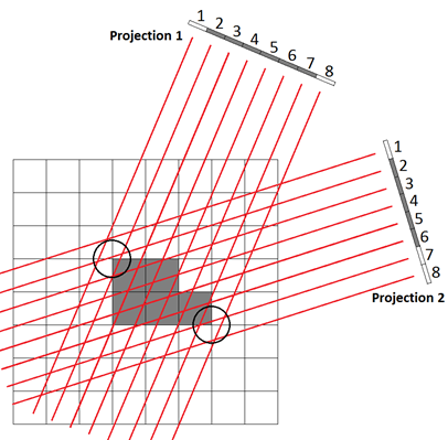
Fig. 7. Inaccuracies in voxel-rays intersections
The figure 7 demonstrates images of some opaque area on 2 projections of input data. Voxel net has some definite state that was reached after a number of iterations. Dark voxels have so high absorption index that even a small intersection with them cause zero resulting intensity. On direction 1 the area occupies pixels 2-7 and on direction 2 – pixels 2-6. The circles mark conflict areas in voxel net. Note that ray 2 from direction 1 intersects the opaque voxel and ray 2 from direction 2 does not. It means that the iteration using direction 2 should increase absorption along the entire ray 2 to compensate the mismatch between current and real projection value. A false stripe of dark voxels appear. Analogically, pixel 7 from direction 2 intersects the dark voxel but the initial data has no absorption on projection here, thus using this ray will make the absorption in previously dark voxel equal to zero.
In such manner two types of artefacts appear near sharp borders: long stripes of false high absorption that are later compensated using other directions and border voxels with false low absorption. Figure 8 shows such stripes on tomography without refraction result (with synthetic data).
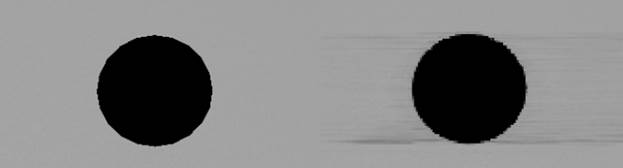
Fig. 8. Initial opaque globe (left) and visualization of tomography result (right)
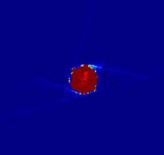
Fig. 9. Horizontal cut of voxel map crossing opaque globe
The limited set of directions makes the problems described above more serious. Figure 9 shows an example of tomography result with taking refraction into account. False trails from opaque areas are oriented along available directions inside the material, usually these are first or last directions visible from one facet. After crossing the gap between available groups of directions the old trails are partially wiped out but the analogic lines for current direction group appear.
5. Proposed method
ART modification is proposed for solving problems of classic methods that is concerned with leaving the linear computation model. Also the modifications necessary for optical data handling are used such as considering refraction.
ART was selected as a base method because it produces the best results from data with opaque areas compared to other methods. Also ART is easy to customize because it is based on some arbitrary correction of desired function along the rays. ART is less sensitive to few projections and discreteness of input data. [3], that’s why it suits the optical tomography problem better .
Input data:
· Set of object photos that is taken from different angles during object 360° rotation around vertical axis
· Geometric photos’ parameters (positions and directions, projection plane size)
· Photo of light source (background model) from the same camera
· Geometric models of scene objects
· Refraction indices of transparent objects
· Size and position of examined volume that is defined with parallelepiped
Result:
· Distribution function of absorption index inside target volume defined on a net
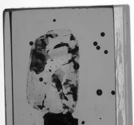
Fig. 10. Example of initial photo: diamond inside immersion glass cube
Input data of optical tomography are not initially suitable for passing them into classic tomography algorithms. We have residual light intensity data in every pixel which depends on initial intensity of light source, absorption in volumetric medium, light energy partition into reflected and transmitted on refractive object surface, light from other light sources.
Figure 10 shows one photo of examined object from a photo sequence taken around it. The cube can be visible on clearance through the front face; a highlight from light source is on the side face.
5.1 Absorption data extraction
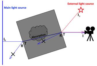
Fig. 11. Forming resulting visible intensity
Figure 11 shows path of the rays with highest impact in
particular pixel’s brightness for a scene with cube. The measured intensity ![]() in camera pixel is:
in camera pixel is:
![]() (4)
(4)
Where
![]() is
irradiated light intensity in current point and direction
is
irradiated light intensity in current point and direction
![]() are
Fresnel coefficients for reflection and transmission respectively, computed for
current incidence angle and material
are
Fresnel coefficients for reflection and transmission respectively, computed for
current incidence angle and material
![]() is
external “parasitic” light intensity. For simplicity in this example let only
the outer cube surface dive gives such reflections.
is
external “parasitic” light intensity. For simplicity in this example let only
the outer cube surface dive gives such reflections.
![]() is
real attenuation coefficient along the ray
is
real attenuation coefficient along the ray
From this expression ![]() can
be evaluated, so it is possible to calculate Radon integral
can
be evaluated, so it is possible to calculate Radon integral ![]() in the exponent:
in the exponent:
![]() (5)
(5)
If the main light source radiation is absorbed totally, then
![]() and
expression under logarithm can become equal to 0 or even negative in case of inaccurate
external light estimation. Adding some rather small constant to term of
fraction or lower limit of fraction can be a solution.
and
expression under logarithm can become equal to 0 or even negative in case of inaccurate
external light estimation. Adding some rather small constant to term of
fraction or lower limit of fraction can be a solution.
5.2 Proposed ART modification
Instead of counting integral value by formula (5) using visible and calculated brightness and then using these values in reconstruction methods, it is proposed to use the visible and calculated brightness itself for absorption correction along the ray.
Let ![]() denote the signed difference between
calculated and visible intensity. Such difference is counted for every sensor
pixel.
denote the signed difference between
calculated and visible intensity. Such difference is counted for every sensor
pixel.
![]() (6)
(6)
Where ![]() is
expected light intensity in sensor pixel considering main light source
intensity, Fresnel coefficients and current absorption index distribution
is
expected light intensity in sensor pixel considering main light source
intensity, Fresnel coefficients and current absorption index distribution
![]() in the
voxel net after applying
in the
voxel net after applying ![]() photos.
photos.
Then using ![]() value the absorption index along the ray
in the net is corrected approximately. The main rule of any correction
is: if
value the absorption index along the ray
in the net is corrected approximately. The main rule of any correction
is: if ![]() then absorption index should increase,
if
then absorption index should increase,
if ![]() then decrease, if
then decrease, if ![]() then it shouldn’t
change.
then it shouldn’t
change.
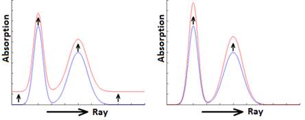
Fig. 12. Additive and multiplicative correction. Initial absorption distribution function along the ray below, corrected distribution above.
![]() (7)
(7)
![]() (8)
(8)
Where ![]() is some coefficient dependent on ray
path length inside the material and specifying algorithm convergence speed.
is some coefficient dependent on ray
path length inside the material and specifying algorithm convergence speed.
Like in classic ART, some empiric methods of correction of absorption distribution along the ray exist. For example, additive correction (7) is constant modification of correction along the ray. Multiplicative correction (8) is modification that is proportional to existing absorption values from previous iteration. Fig. 12 shows changing of absorption distribution along the ray during such corrections. Also a hybrid additively-multiplicative correction was tested and some other corrections with more complex laws.
The correction methods that imply the increasing dependence of correction from existing absorption distribution (for example, multiplicative) partially solve the problem of discretization on the opaque areas’ sharp edges because lower false values of absorption will appear in initially transparent areas.
5.3 Algorithm implementation
First, all the voxel net is initialized with zero value. The algorithm is sequential photos application. A single iteration consists of the following stages:
1) Photorealistic visualization of scene considering current absorption index distribution. It is a first ray tracing step. The following steps are carried out for every ray:
a) Ray-scene intersection
b) Splitting ray into reflected and refracted rays, counting Fresnel coefficients for refracting surfaces
c) Counting current absorption index integral along the ray
d) Ray-light source intersection, acquiring its brightness
e) Resulting brightness calculation, assignment of this value to projection plane pixel
2)
Counting a correction map using visualized image and initial photo form
current direction. It is an image with the same size as photo that contains the
![]() correction
value for each pixel.
correction
value for each pixel.
3) Absorption correction using the correction map. It is a second ray tracing step. The same actions for ray tracing are carried out: ray-geometry intersection and net traversal. Forming the global correction in a separate net.
4) Applying global correction (adding it to the main absorption net)
According to Beer’s law (1) the absorption index is included to exponent. After a number of iterations the absorption index in opaque area becomes high enough to make the transmitted light intensity be close to 0. Due to data discretization, it will be equal to 0, thus it will match the initial data. In this computation model the data with opaque areas become consistent.
The algorithm is implemented on base of ray tracing algorithm. The tomography procedures are built into the single ray tracing process and any configurable ray tracing system is suitable for this purpose. NVidia Optix ray tracing engine was used [9].
The absorption net voxels use float32 data type, one value per voxel. The type and precision selection is caused with comfort and speed of working with floating point values on GPU and also with consideration of correction precision and the fact that initial photos have 8 bit depth. The experiments were carried out where voxels had other data types: for example, 8 and 16 bit with fixed point. They showed that in practice the calculations are possible with 16 bit values minimally though the theoretic minimal voxel bit is higher.
Thus, the voxel net with a size ![]() takes
512 MB of memory. The algorithm requires storing all the voxel net inside video
memory. It takes NVidia GTX 980 GPU 3-5 minutes to finish the calculation with
the following parameters: 400 photos around the object, every photo has 1
megapixel resolution, 1600 iterations or 4 full turns around the object are
performed.
takes
512 MB of memory. The algorithm requires storing all the voxel net inside video
memory. It takes NVidia GTX 980 GPU 3-5 minutes to finish the calculation with
the following parameters: 400 photos around the object, every photo has 1
megapixel resolution, 1600 iterations or 4 full turns around the object are
performed.
6. Results
The proposed algorithm was tested on real data for plotting defect models inside gems. A good result is that during the computation there are no oscillations in absorption index in opaque areas. Fig. 13 shows a horizontal cut of voxel map that was computed from real photos of immersion glass cube with a diamond inside it.
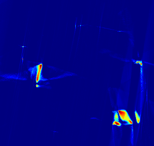
Fig. 13. Result of optical tomography algorithm in one cut of voxel map built from real data (Jet colors)
Also a testing of 2-d version of proposed algorithm on synthetic data without refraction was carried out and a comparison with classic ART was made. The etalon is a cut shown on Fig. 14 where black regions are assumed opaque.
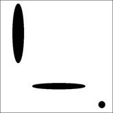
Fig. 14. Etalon for synthetic testing
For clearness, the sequential strategy of projection selection was chosen, moving around the object. Usually, such strategy leads to the fastest convergence of both algorithms (if in case of ART a semi-transparent area is considered)
Several iterations of comparable algorithms are given below by the example of given etalon (Fig. 14) reconstruction. The first is horizontal direction as it one can see on the first iteration. There are 400 projections around the examined area that are distributed regularly. Figures 15 and 16 show 10 full turns around the area.
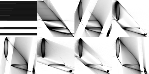
Fig. 15. ART iterations (1, 64, 128, 256, 512, 1024, 2048, 4096)
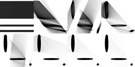
Fig. 16. Proposed algorithm iterations (the same as ART)
Both algorithms – classic ART and proposed method form the images of opaque regions in correct positions on first iterations. But later they work differently: classic ART comes to continuous oscillations of absorption inside the long ellipses and around them (Fig. 15). The proposed algorithm continues converging to some state of voxel map (Fig. 16) that has the following differences from etalon:
- Absolute absorption value in voxels. This happens because the real value of absorption is impossible to be determined using projections. It should be just high enough to consume all light.
- The absorption value in regions that are shadowed with opaque regions from several sides. These areas cannot be reconstructed because of their invisibility on projections.
- Noise that is caused with algorithm imperfection. There are noise “rays” near the opaque regions borders but they are less than in classic ART.
There are some disadvantages of proposed algorithm:
- In case of total light absorption on some region the reconstructed absorption distribution is irregular in this area: lower in center and higher near the border. Classic ART also has such problem.
- Low convergence speed in case of thin and long opaque objects.
- The complete solution to voxel net discretization problem was not found.
7. Conclusion
An optical tomography algorithm based on ART was proposed for reconstructing absorption map inside refractive objects. The new algorithm allows handling refraction, reflection and total light absorption correctly. It was integrated into industrial software for gems cutting and is used for inclusion models plotting inside rough stones.
References
- Afanasyev V.V., Lebedev A.S., Ignatenko A.V. Opticheskaja tomografija prelomljajushhih ob`ektov [Optical tomography of refracting objects]. Proceedings of 17-th seminar “New Information Technologies in Automated Systems” 2014: 185-195 p. [In Russian]
- Bartling, Soenke H., et al. Small animal computed tomography imaging. Current medical imaging reviews vol. 3, no. 1, 2007: 45-59 p.
- Paulus, Michael J., et al. High resolution X-ray computed tomography: an emerging tool for small animal cancer research. Neoplasia vol. 2, no. 1, 2000: 62-70 p.
- Mees, Florias, et al. Applications of X-ray computed tomography in the geosciences. Geological Society, London, Special Publications vol. 215, no. 1, 2003: 1-6 p.
- Natterer, Frank. The mathematics of computerized tomography. Vol. 32. Siam, 1986.
- Gubareni, Nadiya. Vychislitel'nye metody i algoritmy malorakursnoj komp'juternoj tomografii [Algebraic Algorithms for Image Tomographic Reconstruction from Incomplete Projection Data]. INTECH Open Access Publisher, 2009. [In Russian]
- Gordon, Richard, Robert Bender, and Gabor T. Herman. Algebraic reconstruction techniques (ART) for three-dimensional electron microscopy and X-ray photography. Journal of theoretical Biology vol. 29, no. 3, 1970: 471-481 p.
- De Man, Bruno, et al. "Reduction of metal streak artifacts in x-ray computed tomography using a transmission maximum a posteriori algorithm." IEEE transactions on nuclear science vol. 47, no. 3 (2000): 977-981.
- Parker, Steven G., et al. "Optix: a general purpose ray tracing engine." ACM Transactions on Graphics (TOG) vol. 29, no. 4 2010: 66 p.