Optimal filtering of an ordered set of visualization points of road network based on the principles of discrete dynamic programming
, N.А. Kritsyna2, A.K.
Belyakov3Y.V. Borodakiy1
1National Research Nuclear University (MEhPI), Moscow, Russia (115409, Moscow, Kashirskoe highway, 31). e-mail kaf33@mephi.ru
2National Research Nuclear University (MEhPI), Moscow, Russia (115409, Moscow, Kashirskoe highway, 31). e-mail: nak332005@yandex.ru
3National Research Nuclear University (MEhPI), Moscow, Russia (115409, Moscow, Kashirskoe highway, 31). e-mail: belyakov.mephi@gmail.com
Contents
1. Criteria of ordered set of visualization points selection
2. Solution of the criteria minimization problem using discrete dynamic programming method
3. Example of applying of optimal filtration principles with road networks filtering problem
Abstract
The paper focuses on the method of forming the optimal ordered selection of M points from the set of interpolation points of the curve, providing a minimum integral square error in-interpolation. A criterion presented as the sum of private in-integrally criteria is proposed to solve this problem. This approach allows to solve the general problem of optimization-term principle of the discrete Bellman dynamic programming. The proposed method is developed for use in geographic information systems in the formation of databases containing the interpolation points of lines (roads, borders and various other linear objects) for subsequent display on a map as well as the prefiltration of data caused by memory limitations when used in specialized navigation devices.
Keywords: dynamic programming, geographic information system, interpolation, linear object, optimization criterion, graphic representation of solution, solutions hotspots.
Preface
Today various areas of national economic fields widely use geographic information systems for different purposes. As a rule, geographic information systems in the border areas and fronts with various physical processes, the level curves of the terrain, the trajectory of motion of moving objects, road network, etc. are displayed on a map using spline interpolation of the selected order in the ordered set of a large number of points visualization. For example, the road network construction is based on the treatment of information received from the GLONASS satellite navigation system with an interval of 1 second. This information [1] is converted into geocentric coordinates of the current point of the road network and stored in the database of the road network. Obviously, this fractional representation significantly prolongs and complicates the process of following data processing of the road network for future use. Moreover, a lot of this information is redundant and can be derived from the database without the loss of accuracy of the description of the road network. Thus, the task is to have maximum preservation of the original linear degree of curvature of the object at a given level of filtration.
In this context, an important task is to chose an ordered
set of M points of visualization of the initial ordered set of N
points in the visualization, i.e., the forming of ordered set of points ![]() (
(![]() ).
).
1. Criteria of ordered set of visualization points selection
As for the criterion for selecting points, it is rational
to choose the condition of minimization of the surface located between the line
constructed by M ordered points (line![]() ), and a line constructed by N ordered
points (line
), and a line constructed by N ordered
points (line![]() ). This
criterion is equivalent to the integral of square deviation of points from the
line
). This
criterion is equivalent to the integral of square deviation of points from the
line![]() corresponding
points of the line
corresponding
points of the line![]() (Figure
1).
(Figure
1).
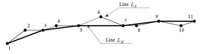
Fig. 1. An example of the formation of the line ![]() . Fox example: N=11, M=6.
. Fox example: N=11, M=6.
Let us assume that ![]() , is the number of points
, is the number of points ![]() between a plurality of
points
between a plurality of
points ![]() , then the
following relations are true:
, then the
following relations are true:
1. ![]() - the first and last points
of the sets
- the first and last points
of the sets ![]() and
and ![]() coinside;
coinside;
2. ![]() - nodes of lines
- nodes of lines ![]() and
and ![]() coinside.
coinside.
Since the nodal points coincide, the total area between the
lines can be presented as the sum of the areas enclosed between nodes. In this
case, the criterion of optimization of points selection in the set ![]() can be written as the sum of
can be written as the sum of
![]()
![]() (1)
(1)
Where ![]()
![]() area of the figure, located
between nodes.
area of the figure, located
between nodes. ![]() .
.
Since the total number of points of ![]() equals M, it is easy to conclude that if
the first
equals M, it is easy to conclude that if
the first ![]() points of the
sequences coinside, the interval between the last points
points of the
sequences coinside, the interval between the last points ![]() and
and ![]() will contain
will contain ![]() points of the set
points of the set ![]() , and vice versa, if the last
, and vice versa, if the last ![]() points in the sequence are the same,
then the interval between the first points
points in the sequence are the same,
then the interval between the first points ![]() and
and ![]() will contain
will contain ![]() points of the set
points of the set ![]() . In addition, the total number of points will
be N. Thus, the restrictions imposed on the argument optimization will
look like:
. In addition, the total number of points will
be N. Thus, the restrictions imposed on the argument optimization will
look like:
![]() ,
, ![]() - a whole number. (2)
- a whole number. (2)
![]() . (3)
. (3)
2. Solution of the criteria minimization problem using discrete dynamic programming method
Representation of criterion (1) as a sum gives the reason to use the principle discrete dynamic programming method [2].
Addressing this optimization problem can be conveniently represented as a graph on a grid bounded solutions (Fig. 2) [3,4].
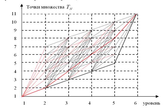
Fig. 2. Example graph for solving the problem with discrete dynamic programming method.
For example: ![]()
Red dotted line marks "conditional" optimal paths, the red line shows the optimal path.
On the horizontal axis we mark the levels of the problem
solutions, the number of levels corresponds to the number of points in the ![]() set. On the vertical axis we
mark the points of the
set. On the vertical axis we
mark the points of the ![]() set,
which can be reached on the i-th level. Obviously, due to limitations of (2)
and (3), each level (except the first and last) comprises
set,
which can be reached on the i-th level. Obviously, due to limitations of (2)
and (3), each level (except the first and last) comprises ![]() dots.
dots.
Since on the first level there is a single point ![]() , the
, the ![]() point of the second level may be
reached only in one way
point of the second level may be
reached only in one way ![]() (Fig.
2). Wherein each point of the level 2 corresponds to area of the figure
(Fig.
2). Wherein each point of the level 2 corresponds to area of the figure ![]() , based on the chord between
two points
, based on the chord between
two points ![]() and
and ![]() (Fig. 1). The values of
these areas are retained.
(Fig. 1). The values of
these areas are retained.
When forming the third level, in every ![]() point of level 3 may be reached in
many ways from the points in level 2 (Fig. 2). In this case, each path
point of level 3 may be reached in
many ways from the points in level 2 (Fig. 2). In this case, each path ![]() will have its own
corrsponding value of sum of surfaces
will have its own
corrsponding value of sum of surfaces
![]() . (4)
. (4)
![]() (5)
(5)
Obviously, the larger the number ![]() , the more paths can lead to this point, and the
more areas of different values will correspond that point. Let us select the
path to the
, the more paths can lead to this point, and the
more areas of different values will correspond that point. Let us select the
path to the ![]() point that
corresponds to the minimum area. To this end, for each point
point that
corresponds to the minimum area. To this end, for each point ![]() we will find such
we will find such ![]() which minimizes the criterion (4),
which minimizes the criterion (4),
![]() ,
,
![]() (6)
(6)
![]() (7)
(7)
The resulting ![]() ,
, ![]() is retained. In the figure the example of the
best ways to points on level 3 are highlighted in red
is retained. In the figure the example of the
best ways to points on level 3 are highlighted in red
The above procedure of forming points of the level 3 is
repeated for levels ![]()
As a result, for the level ![]() we have the following relations:
we have the following relations:
![]() ,
,
![]() (9)
(9)
![]() (10)
(10)
The resulting ![]() ,
, ![]() is retained.
is retained.
The last level M has only one point ![]() , which can reached from a the point
of the prior level
, which can reached from a the point
of the prior level ![]() (Fig.
2). Meanwhile each path
(Fig.
2). Meanwhile each path ![]()
![]() , will have a corresponding
value of the area:
, will have a corresponding
value of the area:
![]() (11)
(11)
We find the only path ensuring the minimum criterion (11):
![]() , (12)
, (12)
![]() (13)
(13)
Using the relations (12), (9) and (6), we follow all the way by the optimum points in the opposite direction:
![]() (14)
(14)
The sequence listed in (14) will be an optimal set of points
of the set ![]() , providing
the minimum criterion (1).
, providing
the minimum criterion (1).
Knowing the number of points ![]() of belonging to the set
of belonging to the set ![]() , it is easy to find the optimum
number of points between nodes
, it is easy to find the optimum
number of points between nodes ![]() , which will no longer be involved in the
process of describing the road network.
, which will no longer be involved in the
process of describing the road network.
To evaluate the effectiveness of the proposed algorithm the set of visualization points was optimized.
Knowing the number of ![]() points of belonging to the set
points of belonging to the set ![]() , it is easy to find the optimal
number of points between the nodes
, it is easy to find the optimal
number of points between the nodes ![]() .
.
A feature of the above method is the maximum preservation of
the original linear degree of curvature of the object at the given filtration
coefficient ![]() .
.
3. Example of applying of optimal filtration principles with road networks filtering problem
The efficiency of the proposed algorithm was investigated on the basis of an ordered sequence of points, represented in OSM [7] in WGS84 format in the form of latitude/longitude (WGS84 is a three-dimensional coordinate system for positioning on the Earth, in which an ellipsoid with a large radius - 6378 137 m (equatorial) and smaller - 6356 752.3142 m (polar) is taken as a basis). Since the selection criterion for points selection is the condition of minimizing the area between the line built by M-ordering chennym points and the line, built on the N ordered points (N> M), it was necessary to calculate the area of arbitrary polygons lying on the ellipse and set points, the geocentric coordinates of which are known.
To solve this problem the coordinates of points are transferred to Mercator coordinates by the formulas [6]:
![]()
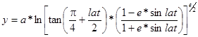 ,
,
where:
- lon/lat - latitude/longitude of the point in radians;
- e - eccentricity of ellipse;
- x, y – Mercator coordinates of the desired point.
As noted above, the criterion of points selection was set to minimize the area between the line constructed by M ordered points of visualization, and the line plotted on the N ordered visualisation points (N> M). Thus, the problem of finding a criterion is reduced to the problem of finding an arbitrary square-foot polygon defined by the coordinates of the vertices. To calculate the area we take an arbitrary point O (for example, the origin). Then the area of the polygon (Figure 3) when traversing vertices in the sequence 1,2, ..., N will be equal to [4]:
![]() ,
,
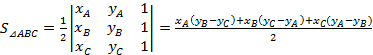 , xi,
yi – Mercator coordinates of the point «i».
, xi,
yi – Mercator coordinates of the point «i».
We can see that ![]() when
traversing vertices counterclockwise and
when
traversing vertices counterclockwise and ![]() clockwise.
Thus, taking into account the signs when adding the areas of triangles, we
obtain the desired area of the polygon.
clockwise.
Thus, taking into account the signs when adding the areas of triangles, we
obtain the desired area of the polygon.
|
|
|
|
Fig. 3. Counting the area of a polygon (not self-intersecting polygon). |
Fig. 4. Counting the area of a polygon (self-intersecting polygon). |

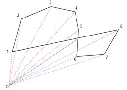
In the case of self-intersecting polygon for each pair of segments the problem of the intersection of two lines is solved. If the intersection point exists, it is determined whether it belongs to the segments forming polygon (Figure 4). Then the self-intersecting polygon is divided at the point of intersection to a non self-intersecting polygons, the area of which is found by the method described above.
We will consider the operation of the algorithm in more details in the example N = 15, M = 7 (Fig. 5).
|
|
|
|
Fig. 5. The initial set of N = 15 visualization points
|
Fig. 6. Formation of points on Level 2 |

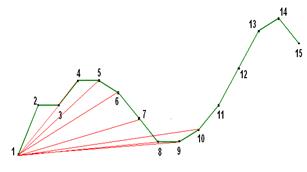
On the first level there is a single point from which points in the second level can be reached by the following method N-M+1= 15-7+1=9 (Figure 6). Each point of the 2nd level has a corresponding area of the figure, based on the chord between the first point and the corresponding point of the 2nd level. These areas are calculated and retained.
When forming the third level, every point of level 3 can be accessed from each point of level 2. Figure 7 shows the possible quasi-optimal ways to the points of level 3 from the points points of level 2. Similar figures can be presented for points 3, 4 , ...,11 in level 2.
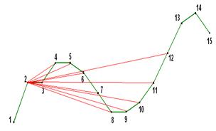
Fig. 7. Formation of conditionally optimal paths on Level 3 for point 2 on Level 2.
Thus, in accordance with formula (4), each path has a corresponding value of sum of the areas of transition from level 1 to level 2 and from level 2 to level 3.
For each point in the 3rd level a path that corresponds to a minimum area must be chosen (see., Relation (6, 7)). As a result we get a set of quasi-optimal ways to level 3.
The last level has only one point, which can be reached from points from the previous level. It is necessary to find the only way providing the minimum criteria.
Going all the way to the optimum point in the opposite direction an optimal set of points, providing a minimum criterion can be found. Representing the solution of the problem in the form of a limited graph on the grid of solutions, we can find the optimal set of points.
For the example reviewed the points are 1, 2, 3, 4, 9, 14, 15 (Fig. 8).
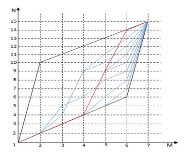
Fig. 8. Graph of solution for the problem. Red line marks the optimal path. Blue lines mark conditionally optimal ways.
Built on the obtained optimal set of points, the curve is
presented in Figure 9. The filtering points error relative to the original
curve at the level of filtering ![]() is Sф=1,1 arbitrary unit
is Sф=1,1 arbitrary unit

Fig. 9. The desired set of M = 7 visualization points, ![]() , Sф = 1,1
, Sф = 1,1
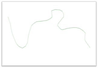
To evaluate the performance of the developed mathematical method and software test calculations for N = 54 were carried out (Figure 10) with the filtration coefficients 2, 3 and 5. The results of the simulation are shown in Figures 11, 12, 13.
|
|
|
|
Fig. 10. An initial set of 54-ordered visualization points |
Fig. 11. |
|
|
|
|
Fig. 12. |
Fig.13. |
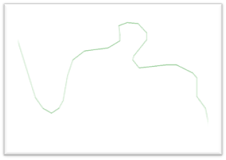
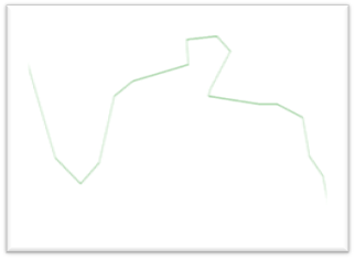
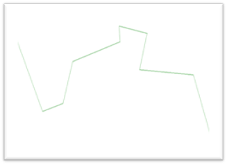
It is obvious that the curvature of the original object is maintained even when reducing the number of points from 54 to 10.
Conclusion
As already noted, the above algorithm can be applied in various information systems for the purpose of filtration of a large amount of data when processing of linear objects, in particular routes (tracks) obtained using automated recording of moving objects (GPS/GLONASS receivers) to reduce time for imaging of linear objects in GIS.
In addition, many specialized navigation devices allow downloading paths (tracks) with a limited number of points (for example, the maximum number of waypoints that can be downloaded in the popular series devices FORE-RUNNER manufactured by GARMIN is 500 points) The above method allows preprocessing the data to be loaded into these devices.
References
- Babich O.A. Information processing in the navigation komplexes. M .: Machine-building, 1991, 512 p.[In russian]
- Kritsyna N.A. Optimization of parameters of the numerical solution of the equations of dynamics. Collection of scientific papers «Algorithms for digital evaluation, monitoring, and managing» ed. By professor Ivashchenko N.N. PhD – M: ATOIZDAT, 1990 – 180 p.[In russian]
- Moiseev N.N., Ivanilov Y.P., Stolyarova E.M. Optimization techniques. - M .: Nauka, 1978.[In russian]
- Sigal I.Kh., Ivanov A.P. Introduction to applied discrete programming: models and computational algorithms: Textbook. - Ed. 2nd, rev. - M .: FIZMATLIT, 2003. - 240 p.[In russian]
- Kleyn F. Elementary mathematics from the point of view of the highest mathemathics: in 2 volumes. T.2.Geometry: Trans. From german. Ed. V.G.Boltyanskogo. - Ed. 2nd. - Moscow: Nauka. Ch. Ed. nat. mat. lit., 1987. – 416 p.[In russian]
- http://wiki.gis-lab.info/ Recalculation of coordinates Lat/Lon in Mercator projection and back.
- http://habrahabr.ru/ The data structure of the project OpenStreetMap.