VISUALIZING THE SENSITIVITY OF THE SOLUTION OF A LINEAR PROGRAMMING PROBLEM WITH FREE PARAMETERS BASED ON DECISION TREE
S.V. Ktitrov, A.A. Kokuyev, Yu.P. Kulyabichev, N.A. Kritsyna, G.A. Gorelkin
National Research Nuclear University "Moscow Engineering Physics Institute", Moscow, Russia
SVKtitrov@mephi.ru, AAKokuyev@mephi.ru, YPKulyabichev@mephi.ru, NAKritsyna@mephi.ru, GorelkinG@yandex.ru
Contents
1. Decision tree for the linear programming problem
3. An example of building a decision tree
4. Decision diagrams for a linear programming problem
Abstract
An approach to sensitivity analysis for solution of a linear programming problem using visual representation of the dependence of the solution of the problem on its parameters is provided. The algorithm of building a decision tree is considered based on which building decision diagrams for the problem was based. The examples of diagrams for problems of different dimension are given.
Keywords: linear programming, simplex method, decision tree, sensitivity analysis, decision diagram
Introduction
Many optimization problems arising, particularly in planning and parametric synthesis of engineering systems, can often be reduced to a linear programming problem. Simplex method, that allows to numerically find optimal solution in a finite number of steps, became a frequent practice to solve these problems. However, in cases where system parameters are specified with a significant error or if the system, an optimal solution for which is sought, is unsteady, the task of determining an optimal solution dependency on one or more varying in predefined range system parameters becomes important. Developed methods for solving such problems, known as sensitivity and solution stability analysis [1,2], solve the problem only for previously obtained optimal solution and are not visual. On the other hand, when formulating a linear programming problems in system parametric synthesis would be immensely useful to have a tool that allows to see dependence of the optimal solution on the initial system parameters, to analyze which constraints are essential and which are irrelevant for a given system parameters variation. Like the phase plane method, applicable for the analysis of solutions of differential equation systems, this tool will ease the analysis and increase the visibility of the analysis results of linear programming problems. To solve this problem the paper suggests the use of decision diagrams, based on decision tree for the linear programming problems with free parameters.
1. Decision tree for the linear programming problem
The problem of linear programming usually is phrased as follows: find the maximum of a function
J(x)=(c,x)
under constraints
![]() (1)
(1)
where x is a vector of variables to be optimized. System matrix of constraints A, vectors of parameters of the objective function c and of the constraints b are usually considered as defined constants. The x vector length is equal to n, the number of constraints is equal to m.
Consider the linear programming problem with free parameters.
Suppose any of the coefficients of the system (1) are not
defined and can vary within the required range ![]() , possibly unlimited.
Then the optimal solution of the system
, possibly unlimited.
Then the optimal solution of the system ![]() , where
, where ![]() is the set
of optimal solutions, can be considered as a result of mapping one-dimensional
region P to
is the set
of optimal solutions, can be considered as a result of mapping one-dimensional
region P to ![]() .
.
General formulation of the linear programming problem with
free parameters assumes that all system parameters (1) are underdetermined.
Then the total number of free parameters of the system will be k=n+n×m+m.
In this case, the range of the parameters![]() is the k-dimensional.
is the k-dimensional.
The solution of this problem can be constructed on basis of
the simplex method as the most worked out and adapted for use with a computer.
Simplex method belongs to a class of search algorithms that implements
consequent walk of vertices of a convex polyhedron formed by the constraints to
achieve an optimal solution. The execution of simplex method steps assumes the
availability of information on a simplex table coefficients balance, based on
which the decision of the bringing one or another vector component into the
basis is made. Suppose that ![]() is not in the basis. If the
decision to bring
is not in the basis. If the
decision to bring ![]() in a basis instead of
in a basis instead of ![]() is taken, then this decision will be correct if the following conditions
is taken, then this decision will be correct if the following conditions
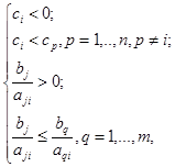 (2)
(2)
which are considered as hypotheses are true. Otherwise, it is necessary to look for another candidate for bringing in a basis, which will necessitate to accept hypotheses similar to (2). Thus, the indeterminancy of one or more parameters results in branching the series of steps of the simplex method.
The total sum of all steps of the simplex method obtained when considering all possible hypotheses about mutual correlation of problem parameters, allows to build a direct graph - a decision tree [3]. There are simplex tables in the nodes of this tree, the edges of the graph are weighted by hypotheses accepted when another simplex table was set. Number of branches of the tree is determined by the number of free parameters of the problem and the given range of change. It should also be taken into account that due to search algorithm of the simplex method one solution can be obtained in different series of steps. The starting basis is also affects the number and location of the tree branches, based on which the obtained tree is not unambiguous, but it contains all of the optimal solutions for the given variation of parameters.
2. Building a decision tree
Building a decision tree especially for problems with lots of free parameters is a time consuming task that requires automation. To accomplish this the authors developed a prototype of a decision tree generation software for the linear programming problems with the free parameters of arbitrary dimensionality.
The software system core is the truth support system of the accepted hypotheses considered when executing simplex method steps. This truth support system is limited, as it does not contain the review mechanism for the truth of accepted assumptions based on new ones, because falsity of previously accepted assumptions can not be identified based on new ones. Contrary to previously accepted assumptions are not considered.
The main purpose of the truth support system is the calculation of contradictions in passed set of assumptions. The passed set of assumptions is a conjunctive normal form.
The algorithms of truth support system are based on converting the set of assumptions from conjunctive normal form into disjunctive normal form and then verifying the truth of each of the conjunctive monomials.
The software package includes the following components:
- software for building a decision tree based on truth maintenance system;
- software for building a graphical representation of a decision tree;
- software that represents decision tree as a set of tables.
3. An example of building a decision tree
Let's consider the example of a decision tree for linear programming problem with two free parameters.
Suppose we want to find the maximum of a function
![]()
under constraints
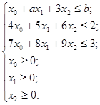 (3)
(3)
In this problem the ![]() and
and ![]() parameters
are chosen to be free. The first three constraints lead to the necessity of
introducing weakening variables
parameters
are chosen to be free. The first three constraints lead to the necessity of
introducing weakening variables ![]() ,
, ![]() and
and ![]() . The first
step leads to hypotheses
. The first
step leads to hypotheses ![]() or
or ![]() when we bring
when we bring ![]() into
the basis. The next steps lead to the building a decision tree. For this
example it is built using the software system developed by the authors. The
final decision tree for the considered problem is shown on fig. 1. Excessive
indexing of free parameters is determined by the features of the developed software.
into
the basis. The next steps lead to the building a decision tree. For this
example it is built using the software system developed by the authors. The
final decision tree for the considered problem is shown on fig. 1. Excessive
indexing of free parameters is determined by the features of the developed software.
As can be seen from the tree, there are 4 variations of the target function values: constant that is independent of the parameters and values that depend on one or two parameters.
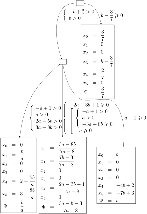
Fig. 1. Decision tree for the problem of dimension 3
4. Decision diagrams for a linear programming problem
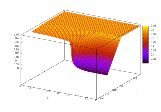
Fig. 2. Dependency diagram of target function against free parameter
The obtained decision tree makes possible to form a diagram family, that allows to visualize the relationship between optimal solution and varying parameters. It should be noted that constraint equations obtained in this way are analytical. The most simple and traditional view has a dependency of the optimum target function value on varying parameters (see fig. 2)
The plot on figure 2 does not allow to distinguish between the areas corresponding the various branches of the decision tree for which the solution has a significantly different nature. To present these areas we can draw a plane projection for the graph on fig. 2 for which we can identify the boundaries based on analytical conditions identified when building the tree. Let's call the suggested projection the decision diagram for a linear programming problem (see fig. 3). There are 6 highlighted areas in figure 3, the area 6 corresponds to no decision.
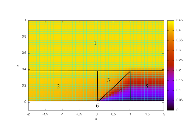
Fig. 3. Decision diagram for the linear programming problem
One of the possible diagram types can be parametric
dependence of the optimal vector components x on varying parameters. In
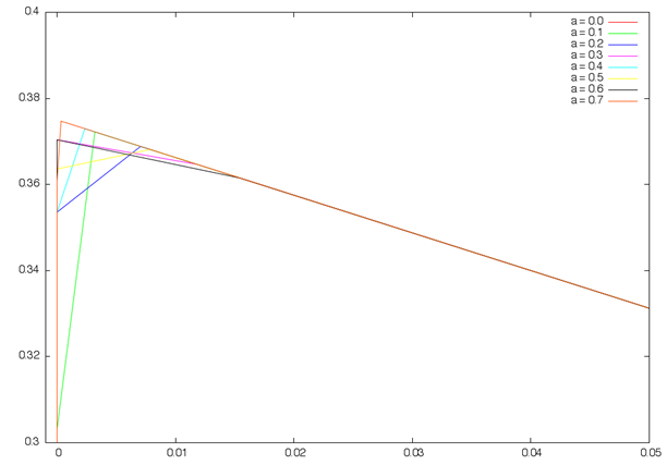
this case one of the parameters can specify the pathway family in space {![]() obtained when changing another parameter. The example of such dependency is
shown in fig. 4, wherein fig. 4a shows a pathway family when fixing parameter
obtained when changing another parameter. The example of such dependency is
shown in fig. 4, wherein fig. 4a shows a pathway family when fixing parameter ![]() and
varying parameter
and
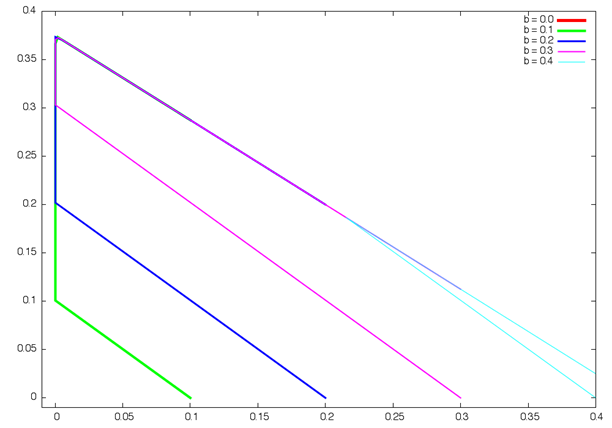
varying parameter ![]() , and fig. 4b shows pathways
when fixing parameter
, and fig. 4b shows pathways
when fixing parameter ![]() and varying parameter
and varying parameter ![]() .
.
a)
b)
Fig. 4. Phase portraits for the linear programming problem
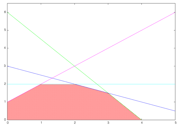
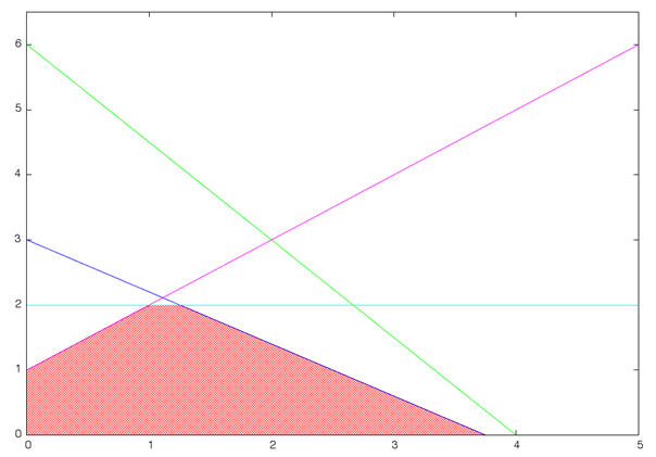
Fig.5. Influence of constraints on optimal solution with varying parameters in constraint
Decision tree at the stage of a system parametric synthesis allows to solve the problem of influence of one or another limitation on the optimal solution.
As can be seen from the diagram shown in fig. 3 for certain values of parameters (areas 1 and 2) the value of the target function does not depend on these parameters. This means that the first constraint including both varying parameters is out of solution forming. Changing the constraint parameter might lead to situation where a limitation is irrelevant at least in a limited range of parameter variation. The non-essential constraints can be determined using the diagram by the lack of influence of the free parameters on the target function value.
Many constraints that determine the optimal solution may vary when there are free parameters in target function coefficients, which is shown in fig. 5. There is a cross section of the simplex formed by constraints together with target function level lines, the slope of which varies depending on the value of free parameter. The corresponding decision tree shown in fig. 6, dependence diagram of the quality criteria against parameters and decision diagram are shown in fig. 7 and 8.
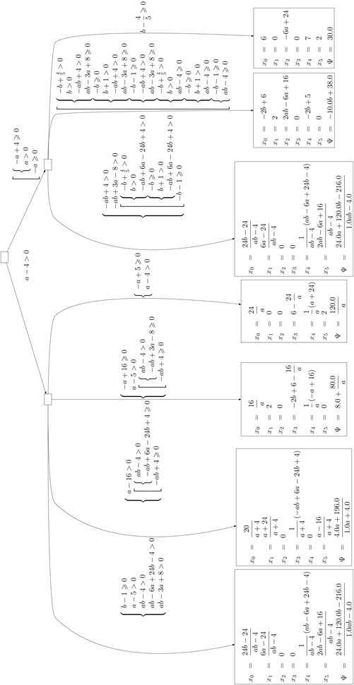
Fig. 6. Decision tree for example 2
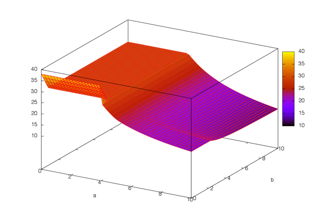
Fig. 7. Dependence diagram of target function against free parameter for the example 2
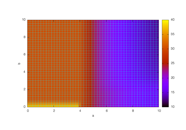
Fig. 8. Decision diagram for the linear programming problem for the example 2
Conclusion
Building a decision tree for linear programming task greatly eases sensitivity analysis of the solution to parameter variations of initial system. The proposed method of visualizing the influence of free parameters at the optimal solution allows to identify the required ranges of initial values accuracy and to cut off the constraints that are irrelevant to a given optimization problem.
This work was financially supported by RFBR (Russian Foundation for Basic Research, РФФИ) within the scientific project No. 13-07-00465A.
References
1. Takha Kh. Introduction to operational research. - 7th ed. - M.: Publishing House. "Williams", 2007. - 912 p.
2. Vasiliev. F.P., Ivanitskiy A.Yu. Linear programing - 3rd rev. Ed. - M.: Factorial Press, 2008. - 328 p.[In russian]
3. A.A. Kokuyev, S.V. Ktitrov. Building a decision tree for linear programming problems. Bulletin of the National research nuclear University "MEPhI", 2014, T.3, No. 1, p. 119-124[In russian]