Starry sky visualiZation
by means of simulation stand
Yu. Kulyabichev, S. Pivtoratskaya
National Research Nuclear University MEPhI (Moscow Engineering Physics Institute), Moscow, Russia
ypkulyabichev@mephi.ru, moeimechko@yandex.ru
Contents
2. Stars detection and classification software
4. Testing the software complex of stars detection and classification on the simulation stand
4.1. Re-calculating the center of the frame
4.2. Estimating errors of the simulation stand
Abstract
This paper is devoted to a software complex of stars detection and classification, as well as its methods and algorithms of image recognition. The use of the software complex for high-precision orientation of small-size spacecraft based on the image of a starry sky's part is described in detail.
The authors consider the method of starry sky visualization by means of a simulation stand “High-Precision Navigating Systems of Small-Size Spacecraft” for testing the software complex. The simulation stand's construction is described, along with the software and hardware for scientific visualization of the starry sky.
The results of testing the software complex by visualizing the starry sky on the simulation stand are given.
Key words: high-precision navigation, pattern recognition, scientific visualization, simulation stand, software complex, starry sky, stars classification, reference star, neighbors.
More than a hundred satellites are launched every year in the world. Each one of them, whatever its purpose – telecommunications, meteorology, navigation or research – carries a system of space orientation. The idea of creating lighter small-size spacecraft from cheaper components is becoming increasingly popular around the world. Reduced mass is achieved by lesser energy consumption, as well as new light and durable materials. Nonetheless, providing sufficient quality of space orientation for a small-size spacecraft is essential. Designing a competitive star tracker also requires developing algorithms of starry sky recognition, because they often operate in outer space, where conditions may be unfavorable and cause disturbances. Researchers often encounter problems trying to project the known test results onto the algorithms in question: free information is mostly superficial and not accurate enough, while devices manufactured by different firms are not identical. Consequently, the best strategy is to conduct preliminary tests of the developed algorithms.
“High-Precision Navigating Systems of Small-Size Spacecraft” – a simulation stand – was created to visualize the starry sky on a monitor on the basis of digital camera pictures containing parts of the starry sky. The stand was used to test and refine the proposed methods and the algorithms of image recognition. A sorted list of stars on the current sky sector served as image data for the test.
The starry sky was projected on the stand with various options: sky’s rotation round the optical axis, interferences from outer space, adjustable number of visible stars.
2. Stars detection and classification software
A software complex for stars detection and classification (SCSDC) was developed to function as an effective tool for high-precision navigation of small-size spacecraft (SSSC) based on pictures of starry sky’s parts [2, 3]. SCSDC uses the studied algorithms to process the pictures taken by a digital camera which contain images of stars.
SSSC move along different trajectories depending on their purposes and functions. Two major groups are found among SSSC: artificial satellites and SSSC designed for flight and research in deep space.
Basic properties of any celestial body – such as position and speed vectors – are calculated indirectly by the use of spherical coordinates, their alteration rate and other parameters. That is why SSSC’s orientation in space relies on the spherical coordinates of the starry sky’s segment in an independent coordinate system calculated with the help of a star tracker attached to the SSSC.
SCSDC determines the orientation of a SSSC by determining the spherical coordinates of the given starry sky segment’s center on the basis of digital pictures of starry sky’s parts.
The coordinates of the given sky sector's center are determined in the following way. There is a digital grayscale picture of a part of the starry sky representing an image – specifically arranged list of stars on the given part of the sky. It is assumed that all stars seen on this sky sector are known to us, because they are listed in the SAO star catalog [4], which is used as basis for all calculations. Next step is to find the best matching list of stars from the star link database by implementing the developed methods and algorithms of pattern recognition for different-type objects. After that, each star from the list is tied to its assigned spherical coordinates (right ascension a and declination d). Finally, the spherical coordinates of the image center are calculated by the method of similar triangles, where two of the identified stars with their known coordinates are chosen as two apices of the triangle while the third apex is the center of the image.
To sum up, the SCSDC makes it possible to determine the inertial orientation of a SSSC in near-earth space and in deep space.
2.1. Methods and algorithms of image recognition on the basis of a structural approach with unified local features
The developed methods and algorithms of starry sky image recognition rest upon a structural approach with the use of unified local features (ULF) of objects [5, 6].
We propose to combine two methods of extracting image features – by an expert and automatically – on different stages of forming the object’s image. An expert’s participation is always advisable for accurate identification of various objects, such as starry sky’s parts, faces etc.
The structural approach stands for describing images in
terms of their parts and relations between them. An image is represented as a
set of simpler images (sub-images) identified by an expert ![]() ,
where xi – sub-image number i (see Figure 1). Further,
each sub-image is repeatedly broken down into smaller sub-images:
,
where xi – sub-image number i (see Figure 1). Further,
each sub-image is repeatedly broken down into smaller sub-images: ![]() .
This procedure is repeated until there are only indivisible sub-images left,
from which local elementary features are extracted.
.
This procedure is repeated until there are only indivisible sub-images left,
from which local elementary features are extracted.
The automatic recognition uses the set of all elementary
features relating to the image: ![]() ,
where fj denotes elementary feature number j.
,
where fj denotes elementary feature number j.
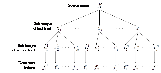
Fig. 1. Hierarchical structure of sub-images of the source image
If all elementary features from the respective set are one by one found in the analyzed picture it means that the image is present in the picture. The structural approach is characterized by the following peculiarities.
Firstly, when dividing an image into several meaningful sub-images the expert does not need to know how their automatic detection is carried out. The recognition procedure uses local elementary features to represent each sub-image extracted by the expert in the way that best suits the algorithms of automatic analysis.
Secondly, representing an image as a structure of sub-images makes the process of detecting the corresponding object in a digital picture more effective.
Thirdly, a large number of images correlates with a small number of recurring elementary features.
Elementary feature is the part of an image which can be in some way separated from neighboring parts. An elementary feature possesses the property of locality and, as a rule, describes changes in one or several image properties in a certain neighborhood. The relevant image properties are: intensity, texture and color. When dealing with monochrome pictures, color is excluded from analysis. There are basically three types of elementary features: blobs, or clusters; edges; interest points, or corners.
Each elementary feature has its own detection method called detector. To recognize an object we apply all the detection methods of elementary features associated with the image to the picture that allegedly contains the image of this object. If most of the features are found in the picture, the image is considered recognized.
In this study we choose the most effective detectors by evaluating their recurrence and information content. We also measure parameters of the areas marked as elementary to build formal descriptions of elementary features called descriptors.
We propose to compare different local features by unifying and placing them in a generalized feature database. Some difficulties may arise because the extracted local features of the same type are usually associated with their own descriptors which may have different dimensionalities. In order to be able to search similar features in the database they are compressed in compact bit vectors of unified format.
For the purposes of the research, descriptors of the three above-mentioned feature types were combined in the proposed binary descriptor. Any feature of each type is stored with 64 bits, thus, the binary representation of each descriptor takes up 192 bits.
We propose to compare the given image with the images of identifiable objects by using a decision rule on the specially packed data from the unified local feature database (ULFdb) of different-type objects. The quality of recognition heavily depends on the sample size of images of identifiable objects in the ULF database. That is why compact data storage and quick feature search are crucially important for the developed database.
Quick search in the ULF database is carried out in two steps:
1. Hashing the ULF database and “rough” similarities search, when the object’s features are compared with ULFs that are cluster centers in the database and matching each feature with one of the clusters.
2. Accurate search of similar features, which compares the object’s features with the features from the matched cluster.
For quick feature search we use hashing – binary coding of database elements – because it allows the use of the Hamming distance, which is calculated much faster than other comparison methods.
Before hashing data, the database is clustered to overcome the inhomogeneity of ULFs’ distribution in n-dimensional space of local features Rn. As the result of clustering, similar features are grouped into one cluster with a single average feature as its center – unified local feature.
In this research we use k-means to cluster the ULF database.
Number of clusters in the proposed algorithm of image recognition is preset and expressed by:
![]() ,
(1)
,
(1)
where ![]() denotes the number of clusters of analyzed
images,
denotes the number of clusters of analyzed
images, ![]() denotes
the cluster of non-images,
denotes
the cluster of non-images, ![]() .
.
The preliminary selection of cluster centers uses a modification of the most effective to date k-means++ algorithm, proposed by Arthur D. and Vassilvitskii C. [7].
Cluster centers are found by minimizing the total distance between each element of the cluster and the closest chosen center. Thus, the formula for the classification center is:
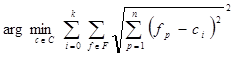 ,
(2)
,
(2)
In the above f denotes a local feature, с is
the cluster center, ![]() are p and i components of the local feature and
the cluster, F is a set of local features, C is a set of cluster
centers, n is the total number of the local feature’s components.
are p and i components of the local feature and
the cluster, F is a set of local features, C is a set of cluster
centers, n is the total number of the local feature’s components.
The number of bits Nb allocated to the cluster center’s hash depends on the number of clusters k as
Nb = 2s ³ k, (3)
where s denotes the calculated integer number.
The hashing is carried out to meet the following condition: cluster centers between which the Euclidian distance is maximal should have the minimal Hamming distance calculated for their hash-values.
The proposed method of image recognition with use of ULF for the accurate comparison of features uses the heuristically found proportion knearest neighbors, which is a ratio of the distance to the nearest neighbor d1 to the distance to the second nearest neighbor d2:
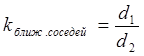 .
(4)
.
(4)
2.2. Implementing methods and algorithms of image recognition for high-precision navigation of small-size spacecraft
The input data for determining the orientation are a digital picture of the starry sky’s part (see Figure 2а). We use the structural approach to look for stars’ elementary features in the picture and then determine the coordinates of the identified stars. Figure 2b shows examples of identified stars.
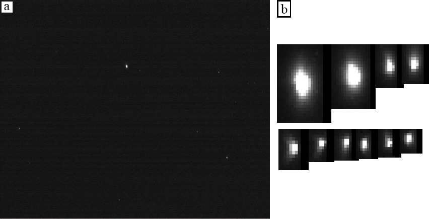
Fig. 2. a) The picture of the starry sky’s part; b) images of detected stars
Determining parameters of pictures of compact objects
The function describing the two-dimensional distribution of brightness in the picture with a luminous point is called point spread function (PSF) [8].
Since the distribution of brightness in the picture is described by a circular two-dimensional Gaussian function, the point spread function:
![]() , (5)
, (5)
where x, y are coordinates of the star in the picture, x0, y0 are coordinates of the star’s image center, а is the parameter of image intensity, s is the parameter of image blur. Thus, the brightness of a given point in the picture is a bilinear convolution, whose kernel is the Gaussian distribution:
 , (6)
, (6)
where I(x0,y0) denotes the function of the initial star brightness, h(x,y) denotes PSF, see (5). In order to determine the PSF one has to obtain parameters x0, y0, a, s.
The image brightness for one pixel is given by:
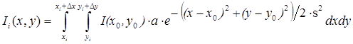 , (7)
, (7)
where i is the pixel’s number, xi, yi denote the coordinates of one of the pixel’s corners, Dx, Dy are pixel sizes along the x and y axes. The unknown parameters of the point spread function can be found after solving (by the method of ordinary least squares) the set of equations (7), constructed for each pixel of the star.
In most cases of broadband emission a point in focus of a camera lens can be approximated by the Gaussian function (Figure 3а), although the PSF is often distorted as a result of optical aberrations characteristic of a given lens. (Figure 3b).
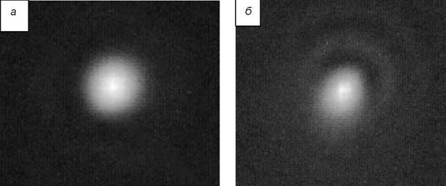
Fig. 3. а) PSF for Pentax C2514-M lenses; b) Fujinon HF25HA-1B lenses
In order to find noisy small circle-shaped areas of light, a special PSF-like filter is built relying on K observations of the luminous point. Using this filter as the kernel for bilinear convolution (6) on each pixel of the found areas in the picture guarantees noise elimination and the best preliminary detection of small circle-shaped areas.
In the developed SCSDC the type of the point spread function is determined on the basis of pictures of relatively bright objects – stars of magnitudes from 2 to 4. This particular interval was chosen because with stars of magnitude greater than 4 we see a PSF-distorting effect of their charge spreading to the neighboring pixels in the points close to the star’s center. The point spread function for stars of magnitude less than 2 may have too few intersections with the edges of the illuminated pixels area and, as a consequence, not enough points for an accurate approximation.
Having selected the most “appropriate” stars, we average the collected values of intensity (PSF-values) to construct a filter with the best PSF. Figure 4 shows the 3d-visualization of the resultant PSF.
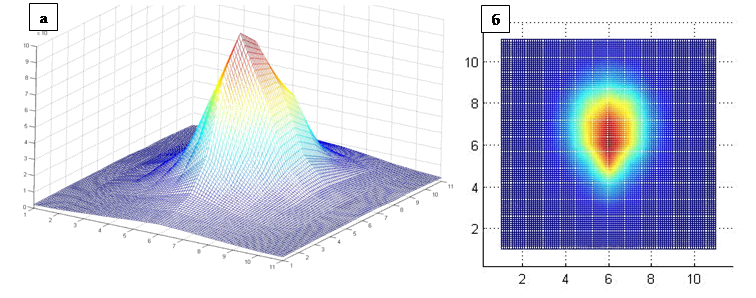
Fig. 4. 3d-visualization of the resultant PSF: a) general view; b) top view
To build the ULF database for stars recognition in the given part of the starry sky we addressed the SAO Star Catalog [4] to create a star link database (SLDB), which would be used for high-precision navigation of small-size spacecraft. The following information about stars was extracted from the catalog: star’s catalog number, right ascension, declination and apparent magnitude. Stars of magnitudes from 0 to 7 inclusive were chosen, totaling up to 15 914 stars.
The Celestial Equatorial Coordinate System [9] was used for starry sky recognition (Figure 5). The fundamental plane in this coordinate system is the celestial equator with the primary direction towards the vernal equinox.
The first coordinate, declination (symbol δ) measures the angular distance from the celestial equator to the observed part of the sky. The declination varies between -90° and 90°, where the part of the sky with с d>0 is to the north of the equator, and the part with d<0 is to the south.
The second coordinate, right ascension (symbol α) is an arc of the celestial equator measured eastward from the vernal equinox ¡ to the declination circle of the center of the observed part of the sky. The ascension varies between 0° and 360° in degrees and between 0h and 24h in hours (360° equals 24h, 1h – 15°, 1m – 15', 1s –15").
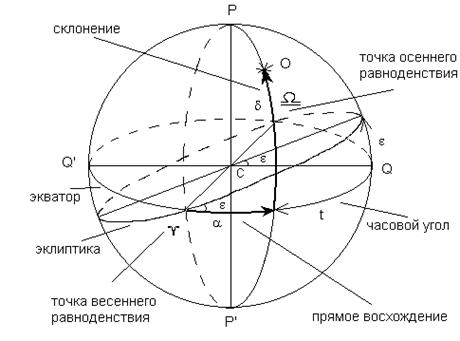
Fig. 5. Celestial
Equatorial Coordinate System.
(Image courtesy of Mashonkina, Sulejmanov, 2003 [9])
While creating the SLDB first to be extracted from the SAO catalog are samples of stars collected according to the rule “‘reference star’ – ‘neighbors’ ”, where the number of neighbor stars does not exceed 32 at the 8° angle of view.
For each “neighbor” star the distance from the “reference” star (in radians) drad is calculated by:
![]() , (8)
, (8)
and the inclination of this distance, α, measured counterclockwise, is calculated by (see Figure 5):
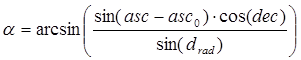 .
(9)
.
(9)
Each cell of the SLDB contains the following properties of the reference star:
- stellar magnitude;
- right ascension;
- declination;
- maximum number of neighbors;
- required number of neighbors;
- tags indicating cells of neighbors;
- list of distances to neighbors;
- list of inclinations of radius-vectors from the reference star to its neighbors;
- SAO catalog number.
This principle enables us to collect samples of all stars in the sphere which comply with the chosen maximum magnitude.
Choosing optimal stellar magnitude
The optimal stellar magnitude was chosen based on the statistical data on the number of “empty” zones, which occur with different settings of number of stars in the preset field of view – 8°. The celestial sphere was divided into overlapping zones 4°×4° with the increment 2° so that the total number of zones was 10588. Table 1 shows the statistics on zones overlap. These statistical data are presented in diagrams (Figures 6, 7), which show that the best ratio of the number of stars to the percentage rate of “empty” zones is found with the stellar magnitude 7,0.
Table 1. Zones overlap
|
Max. stellar magnitude |
Total number of stars |
Rate of “empty” zones, % |
Max. number of “neighbors” |
|
6,0 |
5 092 |
10,72 |
29 |
|
6,5 |
9 023 |
0,85 |
47 |
|
7,0 |
15 914 |
0,028 |
76 |
|
7,5 |
26 559 |
0 |
123 |
|
8,0 |
46 136 |
0 |
206 |
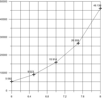
Fig. 6. Total number of stars depending on max. stellar magnitude
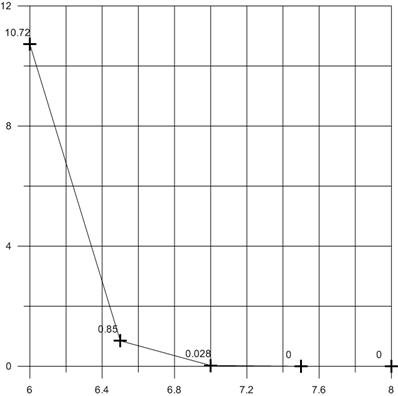
Fig. 7. Number of “empty” zones depending on max. stellar magnitude
If the learning sample contains noise bursts, they might negatively affect the quality of constructing the separating hyperplane. This shortcoming is eliminated by experts correcting the input data.
Determining spherical coordinates of objects
After the previously discussed calculations we have locations of objects in the Cartesian coordinate system, linked to the CCD image sensor. To match these coordinates with the celestial equatorial coordinates it is necessary to obtain the spherical coordinates of stars from the picture in the SLDB.
The process of determining the spherical coordinates of stars with the use of one reference star and calculating the distance and inclination of other stars relative to the reference star is as follows.
As input data we use an arranged list of coordinates of stars in the frame (set of centers of light areas) with rough estimates of their stellar magnitude judging by the size of the light areas. In addition, we have the SLDB, containing links between the reference stars and their neighbors given the preset angle of view.
Thus, the available data for the majority of the stars in the frame are right ascension asc, declination dec, stellar magnitude, x and y in the Cartesian coordinate system, linked to the plane of the image sensor. This data allow us to determine the coordinates ascc, decc of the picture’s center, whose x, y coordinates are known (see Figure 8).
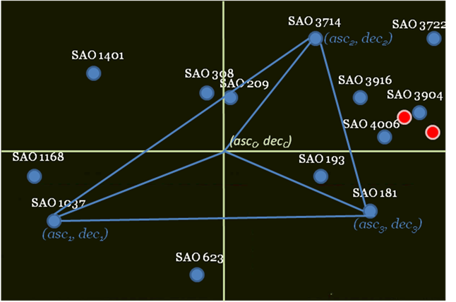
Fig. 8. Determining the coordinates of the frame’s center using the known stars
At the bottom of these calculations lies the formula for determining distances on a sphere. Consequently, the spherical coordinates are given by
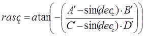 , (10)
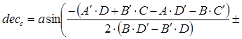
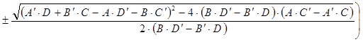 ,
(11)
,
(11)
where
![]() ,
, ![]() ,
, ![]() ,
, ![]() ,
, ![]() ,
, ![]() ,
, ![]() ,
, ![]() ,
,
 ,
,  ,
,  ,
,
dist_koeff – pixels to radians conversion coefficient,
dist_P – distance from the first star to the center of the frame,
dist_P2 – distance from the second star to the center of the frame,
dist_P3 – distance from the third star to the center of the frame,
rasc, dec– spherical coordinates of the first star (right ascension and declination),
rasc2, dec2 – spherical coordinates of the second star,
rasc3, dec3 – spherical coordinates of the third star,
dec_f, rasc_f – spherical coordinates of the center of the frame.
3. Starry sky visualization on the simulation stand “High-Precision Navigating Systems of Small-Size Spacecraft”
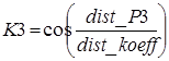
The simulation stand we use for our research consists of 6 parts: a digital camera, a monitor, a computer, an opaque case, computer programs “Recognition of the starry sky’s part” (RSSP) и “Starry sky simulator” (SSS) (Figure 9).
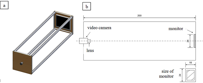
Fig. 9. Design
of the stand “High-Precision Navigating Systems of Small-Size
Spacecraft”: а) general view; b) the stand’s components
For video observation we use a digital video camera “Videoscan-205-USB” with a Navitar TV LENS with the focal length of 50 mm. The camera has a very sensitive CCD (Charge-Coupled Device) and an ADC (Analog-to-digital converter) with an output of maximum 12 bits per pixel. Pixels – light-sensitive elements – are placed on the sensor in the form of an array. The chosen camera is equipped with a 1380*1040 CCD sensor and a lens with a 4° 37′ angle of view.
To get the SCSDC started we need to input data: spherical coordinates and maximal stellar magnitude in the field of view, and check the presence of the SLDB in the program’s directory.
The SSS program is used to project the starry sky’s sector on the monitor (see Figure 10). The projected part of the sky is determined by the coordinates set in the program, and the monitor is parallel to the focal plane of the camera.
Fig. 10. Projection
of the sky’s sector on the image plane. (Image courtesy
of Montenbruck, Pfleger, Astronomy on the personal computer, 1994)
In general, when setting the flight parameters of a satellite it is necessary to model the motion of the stars, so that the sky is moving at a certain speed, corresponding to the desired speed and orbit of the SSSC.
Figure 11 shows the operator interface of the SSS program. Stars are represented by grey dots or circles of various intensities. In the stars’ projection onto the monitor the angular distances between stars are observed.
The camera and the monitor are joined in an integrated measuring system consisting of the SCSDC, guided by the personal computer. This solution helps to collect and evaluate observations automatically.
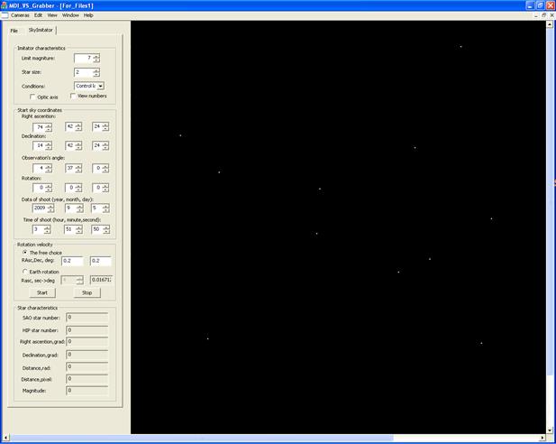
Fig. 11. The interface of the “Starry Sky Simulator” program
The RSSP program reads and processes pictures from the camera. In this program we can set and adjust the exposure time, the interval for retrieving pictures and the name of the recorded image file.
The retrieved frame of the sky is displayed on the observer’s monitor as soon as it is read. Two perpendicular lines are drawn in the picture – they indicate the position of the calculated point.
After the observations one has access to the recorded set of pictures of the starry sky’s parts, as well as to the information about the recognized stars and the coordinates of the given sky sector determined for each frame.
This type of stand is very useful in testing a star tracker, because it helps correct errors in its software, refine the existing algorithms and develop new solutions.
Errors of the RSSP in determining orientation on the stand depend on the precision with which stars are displayed on the digital monitor. The star’s position on the monitor is influenced by the physical properties of the monitor, such as the pixel array and the limited size of the pixels. For these reasons the star is displayed as one pixel or a group of pixels that are the nearest to the given angular direction to the star. The RSSP determines orientation by comparing angular distances between stars in the observed part of the starry sky with the coordinates from the SLDB, therefore, the precision of orientation on the stand depends on the angular size of the monitor’s pixel. Thus, errors in determining orientation on the stand amount to 20 arcsec. in the inertial coordinate system.
The RSSP proves to be robust in determining orientation if the mismatch error between the a priori information about the SSSC’s position in the inertial coordinate system (transmitted from the SSS to the star tracker) and the actual SSS’ orientation in accordance with the displayed part of the sky does not exceed 1°.
Noises on the CCD sensor
Studying a picture obtained from a digital camera, we may notice, apart from stars, randomly located light and dark pixels, as well as local variations of brightness.
Let us examine the main components of noises created by the CCD and the ways to eliminate them [10].
Photon or
shot noise is the noise caused by photon emission. Being a discrete process
it is described by a Poisson distribution with the mean deviation![]() , where
, where ![]() denotes
the photon noise, S is the number of photons falling on one pixel. Despite
the fact that this component is an intrinsic property of light, it is usually
discussed together with other noises occurring on the CCD [11].
denotes
the photon noise, S is the number of photons falling on one pixel. Despite
the fact that this component is an intrinsic property of light, it is usually
discussed together with other noises occurring on the CCD [11].
Dark current is
the noise consisting mainly of thermionic emission; therefore, even an unlighted
image sensor generates a random signal. Since the thermionic emission is a
discrete process, the dark current also obeys a Poisson distribution with the
mean deviation ![]() , where
, where ![]() denotes dark current,
denotes dark current, ![]() is
the number of thermally generated electrons in the general signal. Active
cooling of the CCD sensor helps eliminate this type of noise.
is
the number of thermally generated electrons in the general signal. Active
cooling of the CCD sensor helps eliminate this type of noise.
It is also possible to considerably decrease the impact of dark current by using a dark image. It is deducted from each picture before analysis. To obtain a dark image we need to pixel by pixel average out M frames made with the lens shutter closed and the same exposure as for future frames. The number of M frames is chosen for each individual CCD.
Transfer noise or displacement current occurs during
the transfer of generated charge packets among elements of the CCD. The cause
of this noise lies in the fact that some of the transferred electrons get lost
because of their interaction with randomly located defects and impurities in
silicon. Suppose that each charge packet is transferred independently from
others, then we have the following function for transfer noise: ![]() , where e is
the inefficiency of a separate act of, n is the number of transfers, N
is the number of transferred charges.
, where e is
the inefficiency of a separate act of, n is the number of transfers, N
is the number of transferred charges.
Read noise is the noise occurring when the charge packet is being read from the CCD sensor, converted into electrical current and passes through an amplifier. Read noise can be modeled by a real number R, obeying a Gaussian distribution. Obviously, this basic level of noise is always present in a picture, even if the exposure is set at zero, the sensor is in complete darkness and the noise of the dark current equals zero.
Note that other sources of light signal ambiguity can be ignored, considering the purposes of our research.
Therefore, the function of image brightness ![]() for a picture
obtained from a CCD sensor can be expressed as:
for a picture
obtained from a CCD sensor can be expressed as:
![]() ,
(12)
,
(12)
where I0(x,y) denotes the initial star
brightness, ![]() is photon noise,
is photon noise, ![]() is dark current,
is dark current, ![]() is
transfer noise, R(x,y) is read noise.
is
transfer noise, R(x,y) is read noise.
All components of CCD noises are generated by different physical processes and, therefore, are uncorrelated and independent.
We propose to use the following method of eliminating CCD noises.
First a histogram of pixel intensity for a part of the frame is constructed. Then the left side of the histogram – a certain percentage of the total number of pixels – is clipped off, and the value on the border of the clipping is considered a threshold. All pixels below this threshold are ignored as noise.
Considering small “density” of stars when using a camera lens with the angle of view of 8° (the lighted area of the frame accounts for less than 3% of all frame area), this method proves to be effective.
4. Testing the software complex of stars detection and classification on the simulation stand
4.1. Re-calculating the center of the frame
To determine the precise direction of the axis of sight it
is necessary to correct the coordinates for the center of the starry sky’s part
captured by the camera. The correction is carried out with respect to the center
of the starry sky’s part displayed on the monitor. Before measuring the axis of
sight, two white points A and B (see Figure 12) are displayed on the monitor
with the help of the SSS. Their coordinates are expressed by A = 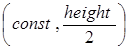 and B =
 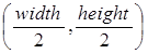 , where width
is the frame’s width, height is the frame’s height, const is the
coordinate of the frame which fulfills the condition
, where width
is the frame’s width, height is the frame’s height, const is the
coordinate of the frame which fulfills the condition ![]() . The coordinates
for the center of the sky’s part equal the coordinates for the point B(xB,yB).
The angle of the frame’s rotation relative to the center is calculated as:
. The coordinates
for the center of the sky’s part equal the coordinates for the point B(xB,yB).
The angle of the frame’s rotation relative to the center is calculated as: 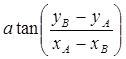 .
.
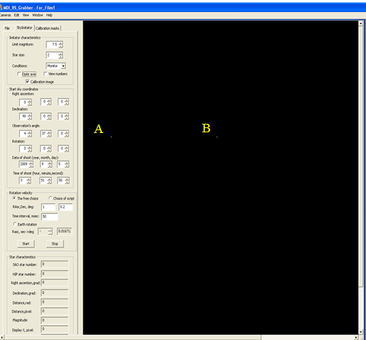
Fig. 12. Checkpoints for determining the center of the frame and the frame’s rotation angle
4.2. Estimating errors of the simulation stand
When testing the SCSDC we need to estimate errors of the created stand. For these purposes we designed several grids of points with known coordinates. These grids are displayed on the monitor with the help of the SSS and are read by the RSSP. Then the RSSP obtains the coordinates for the points from the grid and compares them with the actual coordinates.
We compare the distances between the neighboring vertical and horizontal points in the grid. In theory, these distances should be equal, but in practice there are measurement errors. In this research measurement errors are calculated as a main square deviation from the mean distance.
Types of grids
The grids are numbered according to the order in which they are used. Types of errors identified by grids with lesser numbers are included in the errors identified by grids with greater numbers. Hence, after deducting one by one all grids with lesser numbers from the grid with the greatest number we obtain a relatively “clear” measurement error.
In our case, one pixel of the monitor measures 21,6 arcsec.
Table 2 shows grids for estimating measurement errors. Let us describe them in more detail:
1. For estimating errors in determining star centers in the center and in the corner of the screen.
a) Grid of 11x11 points, increment 10 pixels in the center of the screen.
b) Grid of 11x11 points, increment 10 pixels in the corner of the screen.
2. For estimating errors in displaying stars on the monitor.
Grid of 11x11 points, increment 10,1 pixels in the center of the screen.
3. For estimating optical aberrations (distortion, astigmatism, the vertical incline of the monitor).
Grid of 15x15 points, increment 50 pixels.
4. For estimating the distortion of the projection of star’s location in the sky onto the monitor. In theory, the projection error amounts to 14 arcsec.
Grid of 15x15 points, increment 0,25°.
Table 2. Grids and types of errors
|
Type Grid of error |
1a |
1b |
2 |
3 |
4 |
|
Monitor’s pixels |
- |
- |
X* |
- |
X |
|
Stars’ centers |
X |
X |
X |
X |
X |
|
Distortion |
- |
- |
- |
X |
X |
|
Astigmatism (on the edges) |
- |
X |
- |
X |
X |
|
Vertical incline of the monitor |
- |
- |
- |
X |
X |
|
Projection |
- |
- |
- |
- |
X |
*X- error distorts the grid
Table 3. Parameters of the SCSDC
|
Effectiveness criteria of orientation by sky’s parts |
Attained values of effectiveness criteria |
Required values of effectiveness criteria |
|
Probability of correct star identification, % |
98 |
>95 |
|
Precision of determining orientation, arcsec. |
not less than 20 |
<20 |
|
Permissible angular rate of rotation, deg. per second |
0,05 |
>0,05 |
|
Refresh rate for orientation, Hz |
3-10 |
>1 |
|
Camera’s angle of view, deg. |
8 |
- |
|
Picture size, pixel |
1380*1040 |
- |
|
Maximal stellar magnitude |
7,0 |
6,0 |
|
Size of the star database, units |
15 914 |
<20 000 |
|
Type I error, % |
12 |
<15 |
|
Type II error, % |
26 |
<20 |
The test results give a strong indication that the developed software complex is suitable for high-precision navigation of small-size spacecraft.
5. Conclusion
In this research we conducted the scientific visualization of the starry sky on the simulation stand “High-Precision Navigating Systems of Small-Size Spacecraft” with the help of the specially developed software.
This type of visualization allowed us to thoroughly test the developed methods and algorithms of image recognition. We relied on the structural approach with the use of unified local features to solve the task at hand: recognizing parts of the starry sky and providing high-precision navigation for the small-size spacecraft.
References
1.I. Lisov, Launches: Zapuski: itogi 2010 goda [Summary of 2010]. Novosti Kosmonavtiki [Cosmonautics News], vol. 338, no 3, 2011, pp. 38-39.
2.S.V. Pivtoratskaya, High-precision navigating system for satellite’s orientation in space. 6-th International Conference “Earth from Space – the Most Effective Solutions”, 2011, pp. 364–365.
3.S. Pivtoratskaya, Issledovatelskiy stend «Sistemy vysokotochnoy orientatsii malogo kosmicheskogo apparata» [Experimental stand “High-Precision Navigating Systems of Small-Size Spacecraft”]. Aktualnye problemy rossiyskoy kosmonavtiki: Trudy XXXVI Akademicheskikh chteniy po kosmonavtike [Current Issues of the Russian Cosmonautics: Proceedings of the XXXVI Academic Readings on Cosmonautics]. Moscow, January 2012.
4.SAO Star Catalog Available at: http://tdc-www.harvard.edu/software/catalogs/sao.html
5.S.V. Pivtoratskaya, Yu.P. Kulyabichev. Strukturnyy podkhod k vyboru priznakov v sistemakh raspoznavaniya obrazov [The structural approach to the feature choice for the image recognition systems]. Yestestvennye i Tehnicheskie Nauki (Natural Sciences and Engineering), vol. 54, no 4, 2011, pp. 420–423, 2011.
6.S.V. Pivtoratskaya, Yu.P. Kulyabichev. Ob osobennostyakh strukturnogo podkhoda k raspoznavaniyu obrazov na tsifrovykh izobrazheniyakh. [About characteristics of the structural approach to the image recognition on the digital image]. Vestnik Natsional'nogo Issledovatel'skogo Yadernogo Universiteta “MIFI” (Journal of National Research Nuclear University “MEPhI”), vol. 1, no 1, 2012, pp. 125–128.
7.D. Arthur, S. Vassilvitskii, k-means++: the advantages of careful seeding. Proceedings of the Eighteenth Annual ACM-SIAM Symposium on Discrete Algorithms, 2007, pp. 1027–1035.
8.V.K. Kirillovskij, Opticheskie izmereniya. Chast 4. Otsenka kachestva opticheskogo izobrazheniya i izmerenie ego kharakteristik [Optical measurements. Part 4. Quality evaluation of the optical image and measurement of its characteristics]. Tutorial, SPb, SPbSU ITMO, 2005, p. 67.
9.L.I. Mashonkina, B.F. Sulejmanov. Zadachi i Uprazhneniya po Obschey Astronomii [Tasks and exercises on General Astronomy]. Metodicheskoe posobie k praktikumu po Obschey Astronomii [Study guide to practicum on General Astronomy]. – Kazan, Kazan University, 2003, p. 100.
10.W. Pratt, Tsifrovaya obrabotka izobrazheniy [Digital image processing]. Vol. 2, Мoscow, Mir, 1982.
11.R.E. Bykov, R. Fraer, K.V. Ivanov et al., Tsifrovoe preobrazovanie izobrazheniy [Digital image’s conversion]. Tutorial for universities. Мoscow, Gorjachaja linija-Telekom, 2003, p. 228 p.