NUMERICAL SIMULATION OF TAYLOR–GREEN VORTEX
DECAY IN LAMINAR AND TURBULENT REGIMES
I. Shirokov, T. Elizarova
Moscow State University, Moscow, Russian Federation
Keldysh Institute of Applied Mathematics, RAS, Moscow, Russian Federation
ivanshirokov@inbox.ru, telizar@mail.ru
Contents
Mathematical model and numerical solution method
Comparison of the results for different Re and the energy spectrum
Abstract
We report the results of numerical modeling and visualization for the classical Taylor–Green vortex decay problem basing on smoothed gas dynamic equation system – namely quasi- gas dynamic (QGD) equations for viscous compressible gas flow. QGD system can be obtained by temporal averaging of Navier-Stokes system and differs form it by strongly non-linear terms with the small coefficient that has the dimension of time. The QGD system determines the temporal evolution of the gas density, velocity, and pressure as functions of Eulerian coordinates and time. The temperature, pressure, and density are related by the ideal gas state equation. The Taylor–Green vortex decay is examined for nitrogen at normal temperature with Mach number equal to 0.1. Variations in the Reynolds number are produced by varying the flow density and pressure.
The QGD system is approximated by an explicit time-differencing scheme. All spatial derivatives are approximated by central differences to second-order accuracy, and the time derivatives are approximated with the first-order accuracy. The computation based on the explicit scheme corresponds to the temporal evolution of the gas dynamic flow. The boundary conditions are periodic in three directions, which means that a system of identical Taylor–Green vortices is contained in an unbounded domain. The periodic boundary conditions are implemented by introducing shadow cells adjacent to the physical boundary.
The computations were carried out on the multiprocessor computer system K-100 at the Keldysh Institute of Applied Mathematics of the Russian Academy of Science. The numerical algorithm was parallelized as based on a decomposition of the computational domain by planes x=const with the use of the MPI standard. Our code is portable across different platforms supporting the C language and the MPI standard.
It is shown that QGD equations provide a uniform adequate numerical simulation of both laminar and turbulent evolution of the vortex in a unified manner without varying the parameters of the algorithm. For high Reynolds numbers (Re=1600) numerical results show the transition to turbulence, with the creation of small scale structures accomplished by special evolution of the kinetic energy decay with Kolmogorov scaling of kinetic energy spectrum. For small Reynolds numbers (Re=280 and 100) vortex decay remains laminar. Comparison with reference data show, that for turbulent flow QGD method requires less grid points to achieve the same accuracy compared with different variants of high-order DNS methods. On identical spatial grids at Re=1600, the QGD algorithm was found to be more accurate than the LES method with the Smagorinsky subgrid-scale eddy viscosity model.
The evolution of the vortex flow obtained in the numerical simulation is visualized by depicting the z-component of the vorticity in a 3D domain. Data visualization demonstrates a development of the 3D flow structures and gives opportunity to compare them for laminar and turbulent flow regimes, including a laminar-turbulent transition.
Key words: laminar-turbulent transition, quasi-gasdynamic equations, finite-different schemes, Taylor–Green vortex.
The evolution of a vortex flow defined at the initial time as the Taylor–Green vortex (1937) is an illustrative example of an initially single steady vortex that decays with the formation of a cascade of progressively smaller vortex structures, which in turn gradually decay due to dissipation in the flow. This problem has been well studied theoretically at small Reynolds numbers, when the flow remains laminar, and at high Reynolds numbers, when the initial laminar flow transforms into a turbulent eddy cascade. For this reason, the evolution of the Taylor–Green vortex has been used as a benchmark solution for testing and validation of numerical algorithms designed for turbulent flow simulation (see, for example, [1–5]). A detailed visualization of the numerical results provides more insight into such 3D unsteady processes and ensures their adequate treatment.
In this study, we examine the capabilities of the quasi-gasdynamic (QGD) equations as applied to laminar-turbulent transition modeling in the Taylor–Green flow. Methods for constructing the QGD equations and examples of their use can be found, for example, in [6–8] and more recent publications. Some numerical results concerning laminar-turbulent transition simulation based on the QGD equations were presented in [9–13]. The effect of QGD dissipation on the spectral characteristics of the turbulent flow developing in the decay of a 3D vortex was examined in [14]. Additionally, an algorithm for constructing kinetic energy spectra was described in detail and the accuracy of the numerical simulation of this problem in the case of mesh refinement and a varying relaxation parameter was discussed.
In this paper, the QGD equations are used to compute the decay of the Taylor–Green vortex in nitrogen at normal temperature. Variations in the Reynolds number are produced by varying the flow density and pressure. The numerical results are compared with reference data in laminar (Re=100 and Re=280) and turbulent (Re=1600) vortex decay regimes. Inspection of the numerical results shows that the decay of the initial vortex flow is accompanied by the generation of multiscale vortex structures and their nonlinear interaction. Subsequently, these vortices decay. Additionally, the differences between the vortex structures in laminar and turbulent flow regimes and the moment at which a developed turbulent flow is formed at Re=1600 can easily be seen. The numerical results presented below were obtained on the K-100 multiprocessor computer system [15].
It is well known that the numerical simulation of 3D unsteady flows on multiprocessor computer systems produces large amounts of data, which can hardly be analyzed without using a suitable visualization procedure [16]. In this study, the main goal of flow visualization is to depict vortex structures in a 3D flow field, to keep track of their temporal evolution and transformations, and to compare vortex structures in various flow regimes. The last goal is achieved with the help of TecPlot visualization software. An analogous numerical approach and similar software tools were used earlier to compute free-surface flow oscillations in a tank subject to nonuniform movements [17].
Following [3], we consider a cubical domain ![]() in Cartesian coordinates, where
in Cartesian coordinates, where
![]() m. The domain is filled with a gas (nitrogen). The state of the gas
is described by the following variables:
m. The domain is filled with a gas (nitrogen). The state of the gas
is described by the following variables: ![]() is the density,
is the density, ![]() ,
, ![]() ,
, ![]() are the components of the macroscopic
gas velocity, and
are the components of the macroscopic
gas velocity, and ![]() is the pressure. The velocity components are collectively
denoted by
is the pressure. The velocity components are collectively
denoted by ![]() (similar notation is used for other vectors
and tensors).
(similar notation is used for other vectors
and tensors).
As is customary, the initial flow field for the Taylor–Green vortex is given by (see [1])
![]() ,
, ![]() ,
, ![]() ,
,
![]() . (1)
. (1)
The initial temperature distribution is uniform in
space: ![]() K. The initial density is determined by the ideal gas equation of state:
K. The initial density is determined by the ideal gas equation of state:
![]() . (2)
. (2)
The gas constant for nitrogen is R=297 J/(kg·K). Note that the initial flow parameters ![]() ,
, ![]() , and
, and ![]() are also related by
the equation of state
are also related by
the equation of state ![]() . The initial Mach number is defined as
. The initial Mach number is defined as
![]() , (3)
, (3)
where the speed of sound in nitrogen under
the initial conditions is ![]() m/s and the
specific heat ratio is
m/s and the
specific heat ratio is ![]() [18]. Since the Mach number in the problem is low, the flow can be considered
weakly compressible [3].
[18]. Since the Mach number in the problem is low, the flow can be considered
weakly compressible [3].
The Reynolds number is defined as
![]() , (4)
, (4)
where
![]() kg/(m·s) is
the dynamic viscosity of nitrogen at the temperature
kg/(m·s) is
the dynamic viscosity of nitrogen at the temperature ![]() K [19]. Below, the flows computed at Re=100, Re=280, and Re=1600 are compared with the reference data from [1], [4], and [3],
respectively. In [2] a similar problem of isotropic turbulence decay was solved
in the inviscid case by applying five high-order accurate finite-difference algorithms
in the LES
approximation, namely, Jameson's
multistage scheme, Roe-TVD-MUSCL scheme, and various ENO schemes.
K [19]. Below, the flows computed at Re=100, Re=280, and Re=1600 are compared with the reference data from [1], [4], and [3],
respectively. In [2] a similar problem of isotropic turbulence decay was solved
in the inviscid case by applying five high-order accurate finite-difference algorithms
in the LES
approximation, namely, Jameson's
multistage scheme, Roe-TVD-MUSCL scheme, and various ENO schemes.
The initial values are specified in the
following order. The initial characteristic velocity ![]() is determined by (3); the density
is determined by (3); the density ![]() , by (4); and the pressure is given by
, by (4); and the pressure is given by ![]() . Then the initial distributions of velocity and
pressure are specified using (1) and the initial density distribution is given
by (2).
. Then the initial distributions of velocity and
pressure are specified using (1) and the initial density distribution is given
by (2).
The boundary conditions are periodic in three directions, which means that a system of identical Taylor–Green vortices is contained in an unbounded domain.
Mathematical Model and Numerical Solution method
The gas flow is governed by the
macroscopic system of QGD equations [8]. This system determines the temporal evolution of the gas density, velocity, and pressure as functions of Eulerian
coordinates and time. The temperature, pressure, and density are related by the ideal gas equation of state (2). The
total energy per unit volume E and the total specific enthalpy H are calculated using the formulas ![]() and
and ![]() , where
, where ![]() is the specific heat ratio.
is the specific heat ratio.
In Cartesian coordinates, the QGD system is written as [8, p. 94]
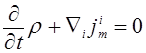 ,
(5)
,
(5)
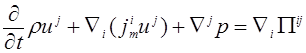 , (6)
, (6)
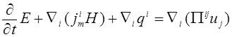 . (7)
. (7)
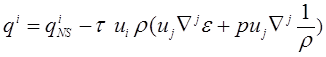
The mass flux density ![]() is determined as follows [8, p. 97]:
is determined as follows [8, p. 97]:
![]() ,
, ![]() . (8)
. (8)
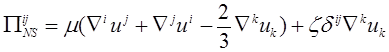
The viscous stress tensor ![]() and the heat flux
and the heat flux ![]() are given by [8, pp. 83, 96]
are given by [8, pp. 83, 96]
 , (9)
, (9)
 , (10)
 ,
, ![]() . (11)
. (11)
Here, ![]() is the Kronecker delta (
is the Kronecker delta (![]() for
for ![]() and
and ![]() for
for ![]() ) and
) and ![]() is internal energy per unit mass. The thermal conductivity is
given by the relation [8, p. 71]
is internal energy per unit mass. The thermal conductivity is
given by the relation [8, p. 71]
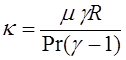 ,
(12)
,
(12)
where Pr is the Prandtl number. In the problem under study, Pr=0.71 [3].
The dynamic viscosity ![]() involved in expressions (9)–(11) for
involved in expressions (9)–(11) for ![]() and
and ![]() is defined as a function of temperature [18]:
is defined as a function of temperature [18]:
![]() , (13)
, (13)
where ![]() describes the intermolecular interaction in the gas. In this study, we use
describes the intermolecular interaction in the gas. In this study, we use ![]() [16]. The volume viscosity is set to zero according to [3]:
[16]. The volume viscosity is set to zero according to [3]: ![]() .
.
The relaxation parameter ![]() involved in (8)–(11) is defined as
involved in (8)–(11) is defined as
![]() , (14)
, (14)
where ![]() is the local speed of sound and h is the spatial mesh size. The terms containing the coefficient
is the local speed of sound and h is the spatial mesh size. The terms containing the coefficient ![]() represent subgrid dissipation, which
smoothes out fluctuations of gasdynamic variables on scales on the order of the
mesh size. The coefficient
represent subgrid dissipation, which
smoothes out fluctuations of gasdynamic variables on scales on the order of the
mesh size. The coefficient ![]() can be regarded as a tuning parameter determining the
degree of subgrid
dissipation.
can be regarded as a tuning parameter determining the
degree of subgrid
dissipation.
To solve problem (5)–(14) with initial conditions (1)
by a finite-difference method, in the domain ![]() we introduce a uniform grid in space and time:
we introduce a uniform grid in space and time: ![]() ,
, ![]()
![]() ,
, ![]()
![]() ,
, ![]()
![]() ,
, ![]()
![]() .
Note that the number
.
Note that the number ![]() of time steps is not fixed prior to the computations. For all gasdynamic quantities depending on
coordinates, we introduce grid functions, for example, for density,
of time steps is not fixed prior to the computations. For all gasdynamic quantities depending on
coordinates, we introduce grid functions, for example, for density, ![]() and likewise for the other variables. The
dimensions of the grid functions are the same as those of the corresponding
physical quantities.
and likewise for the other variables. The
dimensions of the grid functions are the same as those of the corresponding
physical quantities.
The problem is approximated by an explicit time-differencing scheme. All spatial derivatives are approximated by central differences to second-order accuracy, and the time derivatives are approximated to first-order accuracy. The algorithm for constructing the difference scheme is the same as in [11–14]. The computation based on the explicit scheme corresponds to the temporal evolution of the gasdynamic flow. The periodic boundary conditions are implemented by introducing shadow cells adjacent to the physical boundary. Then, for example, a grid with N=130 is denoted as 1283 (i.e., the shadow cells are not taken into account).
The initial free path of gas molecules is defined as ![]() , where
, where ![]() [16]. In the mathematical
model used, it is required that
[16]. In the mathematical
model used, it is required that ![]() . This condition was satisfied in all the computations presented below.
. This condition was satisfied in all the computations presented below.
The time step is determined by the Courant condition [8, p. 140]: ![]() , where
, where ![]() is the Courant number. Note that
is the Courant number. Note that ![]() is involved in expression (14) for
the relaxation parameter
is involved in expression (14) for
the relaxation parameter ![]() .
.
As in [11–14], the computations were performed
in dimensional variables. To compare the numerical results with reference data,
the former were nondimensionalized using the reference parameters ![]() ,
, ![]() , and
, and ![]() . Accordingly, the nondimensional time is given by
. Accordingly, the nondimensional time is given by ![]() , where
, where ![]() s, and the nondimensional kinetic
energy per unit volume is
s, and the nondimensional kinetic
energy per unit volume is ![]() .
.
The evolution of the vortex flow obtained in the numerical simulation is visualized by depicting the z-component of the vorticity in a 3D domain. Vorticity visualization is conventional in the study of the Taylor–Green flow problem [1–3]. It provides an illustrative representation of the flow structures under study and makes it possible to compare numerical results with reference data.
The computations were carried out on the multiprocessor computer system K-100 at the Keldysh Institute of Applied Mathematics of the Russian Academy of Science. The numerical algorithm was parallelized as based on a decomposition of the computational domain by planes x=const with the use of the MPI standard. This technique has been successfully applied in [11–14]. Note that our code is portable across different platforms supporting the C language and the MPI standard.
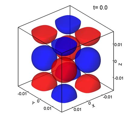
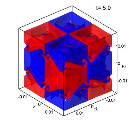
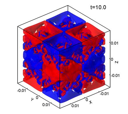
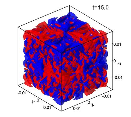
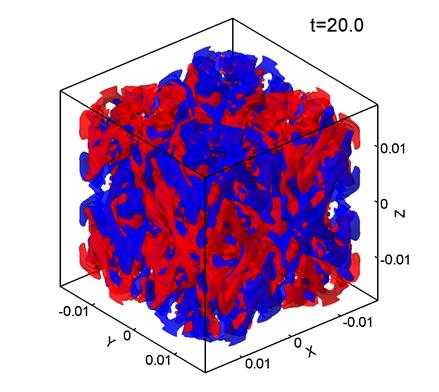
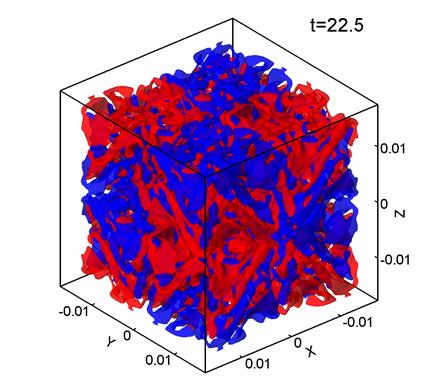
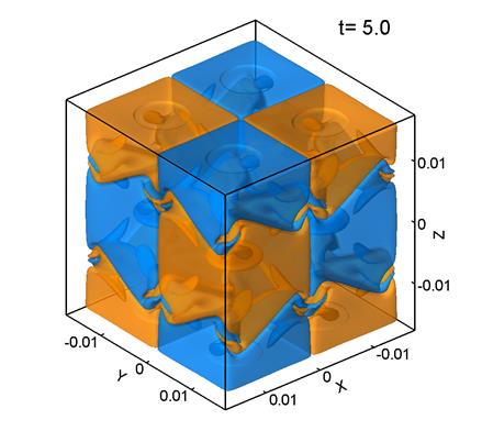
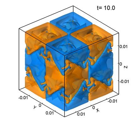
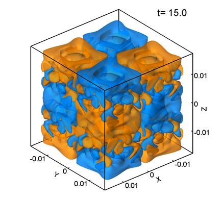
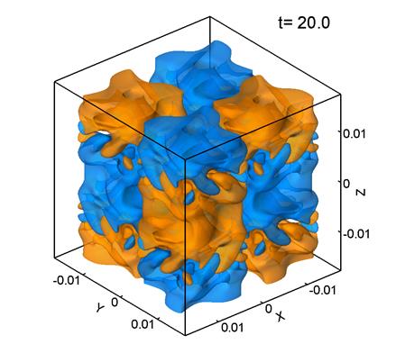
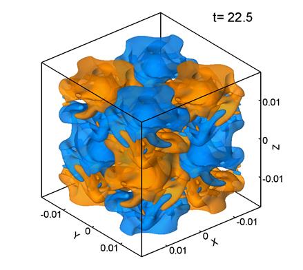
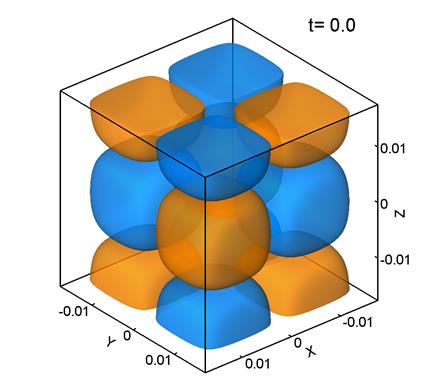
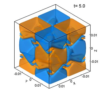
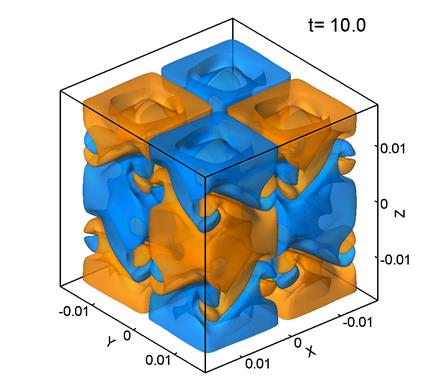
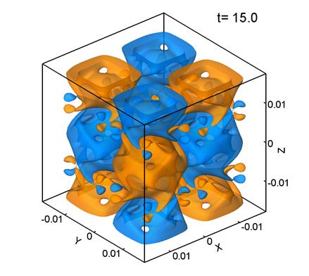
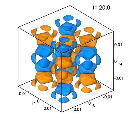
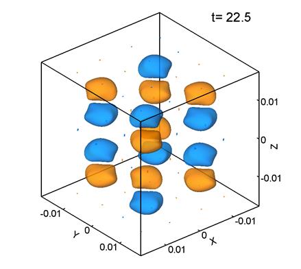
Figure 1 shows level surfaces
(isosurfaces) of the
![]() -component of vorticity, i.e., the z-component of
the curl of the velocity field:
-component of vorticity, i.e., the z-component of
the curl of the velocity field:
![]() .
.
Note that ![]() was computed
in dimensionless form. The level surfaces are presented for a sequence of dimensionless
times from t=0 to t=22.5. The red
color corresponds to Vz=0.7, and the blue color, to Vz=-0.7. Here,
the grid consists of 1283
points, the mesh size is
was computed
in dimensionless form. The level surfaces are presented for a sequence of dimensionless
times from t=0 to t=22.5. The red
color corresponds to Vz=0.7, and the blue color, to Vz=-0.7. Here,
the grid consists of 1283
points, the mesh size is ![]() m, and
m, and ![]() .
.
(a) (b)
(c) (d)
(e) (f)
Fig. 1.
It can be seen that the initially regular velocity distribution (1) (Fig. 1a) breaks up into smaller structures. At the times t=5 and 10 (Figs. 1b, 1c) the velocity distribution retains some features of the
initial Taylor–Green vortex, but by t=15 (Fig. 1d) the
flow becomes chaotic with nearly no relation to the initial vortex structure. This chaotic velocity distribution is
typical of turbulent flows. This flow evolution agrees well with the Taylor–Green vortex
evolution observed at Re>500 in [1] and at Re=1600 in [3, 5]. Note that the dimensionless time interval ![]() corresponds to the characteristic period
of rotation of the initial vortex (1).
corresponds to the characteristic period
of rotation of the initial vortex (1).
(a) (b)
Fig. 2,
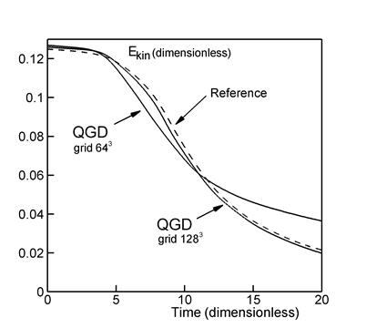
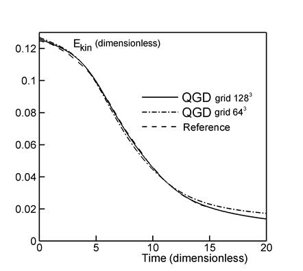
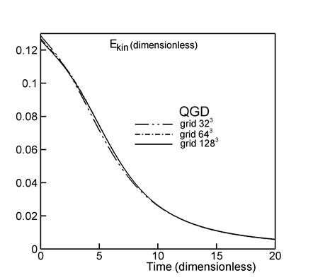
Figure 2a shows the temporal evolution of the
kinetic energy per unit volume averaged over the computational domain ![]() :
:
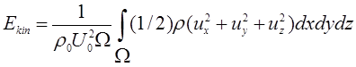 .
.
The kinetic energy and time are
represented in dimensionless units. The solid curves depict our results obtained
on a grid consisting of 643 points with ![]() m and on a grid of 1283 points with
m and on a grid of 1283 points with ![]() m,
m, ![]() . The dashed curve shows the reference data from [3] produced
by a dealiased pseudospectral method and various discontinuous Galerkin methods.
. The dashed curve shows the reference data from [3] produced
by a dealiased pseudospectral method and various discontinuous Galerkin methods.
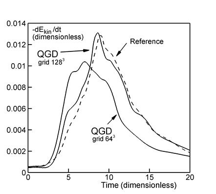
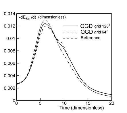
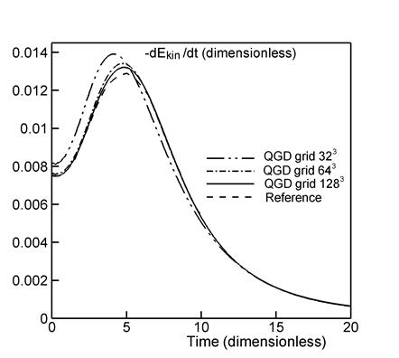
Figure 2b displays
the kinetic energy dissipation rate ![]() as a function of time. As in Fig. 2a, the solid curves depict our results, while the dashed curve shows the reference data from [3]. The maximum value of the dissipation rate indicates the laminar-turbulent transition
and the formation of the Kolmogorov–Obukhov spectrum (Fig. 6). Figure 2 shows that the results obtained on the
finer grid are much more similar to the reference data than those on the
coarser grid.
as a function of time. As in Fig. 2a, the solid curves depict our results, while the dashed curve shows the reference data from [3]. The maximum value of the dissipation rate indicates the laminar-turbulent transition
and the formation of the Kolmogorov–Obukhov spectrum (Fig. 6). Figure 2 shows that the results obtained on the
finer grid are much more similar to the reference data than those on the
coarser grid.
According to the numerical results
obtained for ![]() in [14],
an increase in the coefficient
in [14],
an increase in the coefficient ![]() from 0.1 to 0.9 leads to
smoother plots of
from 0.1 to 0.9 leads to
smoother plots of ![]() and to the maximum of
and to the maximum of ![]() shifted toward earlier times. A similar
effect is observed with a decreasing number of spatial grid points.
shifted toward earlier times. A similar
effect is observed with a decreasing number of spatial grid points.
DNS simulations of the Taylor–Green flow have been presented in a number of studies, for example, in [1, 3–5]. Specifically, the computations in [5] were preformed on a grid consisting of 2563 nodes by applying methods of high-order accuracy in time and space. The number of nodes used in these computations was estimated as the minimum possible one required for the vortex structures corresponding to a given Reynolds number to be well resolved by applying the DNS approach. The results produced by the QGD algorithm on a 1283 grid (Fig. 2) agree well with the data of [1, 5] obtained on a 2563 grid.
The LES approach allows one to reduce the number of computational nodes in the numerical algorithm. The flow simulation based on the LES method employing the Smagorinsky filtering model with 643 nodes is presented in [5]. According to these results, the maximum dissipation rate is understated and reaches values of ~ 0.006, while the reference value is ~ 0.012. Thus, the Smagorinsky LES model is too dissipative for the Taylor–Green vortex flow. Note that a dynamic variant of the Smagorinsky model is used in [5], in which case the magnitude of subgrid dissipation is automatically adapted to the resolved scales in the flow. The QGD algorithm on a 643 grid gives a maximum dissipation rate of ~ 0.01 (Fig. 2b).
Figure 3 shows
level surfaces of the ![]() -component of vorticity. The yellow color corresponds to Vz=0.2,
and the blue color, to Vz=-0.2. Here, the grid consists of 1283 points, the mesh size is
-component of vorticity. The yellow color corresponds to Vz=0.2,
and the blue color, to Vz=-0.2. Here, the grid consists of 1283 points, the mesh size is ![]() m, and
m, and ![]() .
.

(a) (b)
(c) (d)
(e) (f)
Fig. 3.
Inspection of Fig. 3 reveals that the velocity field at Re=280 preserves the general character of the initial regular distribution, although relatively small structures are generated. In this case, the flow pattern becomes partially turbulent.
(a) (b)
Fig. 4.
Figure 4 displays the temporal evolution of (a) the kinetic energy ![]() and (b) its dissipation rate
and (b) its dissipation rate ![]() at Re=280. The solid and dash-dotted curves depict our results, while the dashed
curves show the reference data from [4] produced by the Fergus pseudospectral code and a discontinuous Galerkin
method with 963 degrees of freedom. The number
of computational points in the QGD algorithm is 643 (with
at Re=280. The solid and dash-dotted curves depict our results, while the dashed
curves show the reference data from [4] produced by the Fergus pseudospectral code and a discontinuous Galerkin
method with 963 degrees of freedom. The number
of computational points in the QGD algorithm is 643 (with ![]() m, dash-dotted curve) and 1283 (with
m, dash-dotted curve) and 1283 (with ![]() m, solid curve); in both cases,
m, solid curve); in both cases, ![]() . As in the case of Re=1600, the results on the finer grid are closer to the
reference data than those on the coarser grid, although the differences at Re=280
are rather small.
. As in the case of Re=1600, the results on the finer grid are closer to the
reference data than those on the coarser grid, although the differences at Re=280
are rather small.
Figure 5 presents
level surfaces of the ![]() -component of vorticity computed at Re=100. Here, the grid consists of 1283 points, the mesh size is
-component of vorticity computed at Re=100. Here, the grid consists of 1283 points, the mesh size is ![]() m, and
m, and ![]() .
.
(a) (b)
(c) (d)
(e) (f)
Fig. 5.
(a) (b)
Fig. 6.
Figure 6b shows the temporal evolution of
the kinetic energy and its dissipation rate ![]() computed
on three grids consisting of 323
points (with h=10-3 m), 643 points (with
computed
on three grids consisting of 323
points (with h=10-3 m), 643 points (with ![]() m), and 1283
points (with
m), and 1283
points (with ![]() m),
m), ![]() . As in the case of Re=280, the numerical results obtained on the finest grid
are closer to the reference data than those produced on the coarser grids. The
reference profile (dashed curve) was given in [1]. Note that the laminar Taylor–Green flow at Re=100 can be fairly well
simulated even on the very coarse grid with 323
nodes.
. As in the case of Re=280, the numerical results obtained on the finest grid
are closer to the reference data than those produced on the coarser grids. The
reference profile (dashed curve) was given in [1]. Note that the laminar Taylor–Green flow at Re=100 can be fairly well
simulated even on the very coarse grid with 323
nodes.
The maximum value of ![]() for Re=100 occurs at t=4.5. At this
time, the flow still retains some of the initial anisotropy of the Taylor–Green vortex (Fig. 5b). Later,
the flow pattern also remains anisotropic. Thus, the whole decay of the single vortex at Re=100 remains laminar, so that
no chaotic field of small vortices typical of Re=1600 is formed
(Figs. 1d–1f). This pattern of the Taylor–Green vortex decay
agrees with
the data presented in [1] for laminar flows at Re<500.
for Re=100 occurs at t=4.5. At this
time, the flow still retains some of the initial anisotropy of the Taylor–Green vortex (Fig. 5b). Later,
the flow pattern also remains anisotropic. Thus, the whole decay of the single vortex at Re=100 remains laminar, so that
no chaotic field of small vortices typical of Re=1600 is formed
(Figs. 1d–1f). This pattern of the Taylor–Green vortex decay
agrees with
the data presented in [1] for laminar flows at Re<500.
Comparison of the Results for Different Re and the Energy Spectrum
Figure 7 shows the profiles of the
dissipation rate ![]() as a function of time for three Reynolds
numbers: 100, 280, and 1600. Additionally, Fig. 7 presents the reference data from
[1, 4, 3]. As the Reynolds number increases, the maximum of
as a function of time for three Reynolds
numbers: 100, 280, and 1600. Additionally, Fig. 7 presents the reference data from
[1, 4, 3]. As the Reynolds number increases, the maximum of ![]() shifts to the right. The results obtained at
Re=100 and 1600 are
in quantitative agreement with the corresponding curves plotted in Fig. 7 in [1], which were computed on a grid with 2563
points by applying the DNS approach.
shifts to the right. The results obtained at
Re=100 and 1600 are
in quantitative agreement with the corresponding curves plotted in Fig. 7 in [1], which were computed on a grid with 2563
points by applying the DNS approach.
Note that the QGD model used does not require any modification or parameter tuning in the transition from laminar to turbulent flows. All variants are computed in a unified manner.
Figure 8 shows the spectral density of
kinetic energy at Re=1600
calculated using the same technique as in [14]. Additionally, Fig. 8 presents a
line with a Kolmogorov slope of -5/3. The spectrum was calculated at the time t=8.5,
when ![]() reaches its maximum value (Fig. 2b). The
energy spectrum profile is similar to that for Re=1600 plotted in Fig. 4 in [4] and to the profile for Re=1500 presented in Fig. 8.3 in [5]. The spectra in Fig. 8 were computed on grids with 643 and 1283 points.
It can be seen
that the energy profiles obtained on both grids are fairly similar, which
suggests that the turbulent smoothing is physically adequate. As the number of grid points increases, the spectral density curve becomes
smoother and approaches the -5/3 line.
reaches its maximum value (Fig. 2b). The
energy spectrum profile is similar to that for Re=1600 plotted in Fig. 4 in [4] and to the profile for Re=1500 presented in Fig. 8.3 in [5]. The spectra in Fig. 8 were computed on grids with 643 and 1283 points.
It can be seen
that the energy profiles obtained on both grids are fairly similar, which
suggests that the turbulent smoothing is physically adequate. As the number of grid points increases, the spectral density curve becomes
smoother and approaches the -5/3 line.
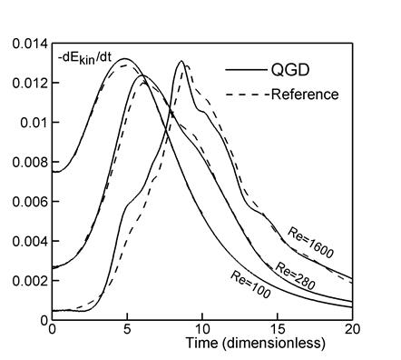
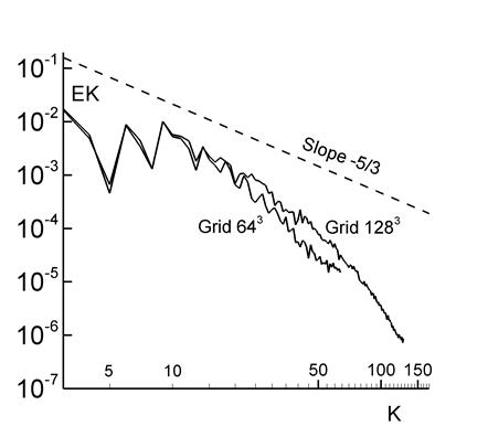
Fig. 7. Fig. 8.
Figure 9 shows streamlines and contours of the vorticity Vz in the plane z=0.008 m for (a) Re=1600 and (b) Re=100 at t=20. A developed vortex flow pattern is observed at Re1600, while at Re=100 no small vortex structures are seen. Moreover, the value of Vz at Re=1600 is much higher than that at Re=100. Thus, the difference between the turbulent and laminar cases is easily seen. The symmetry of the computed solution in Fig. 9 is the same as in initial conditions (1), which suggests that the numerical algorithm is correct and stable.
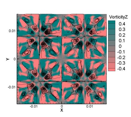
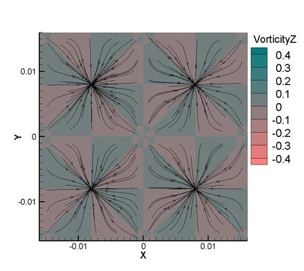
(a) (b)
Fig. 9.
The DNS approach was used to simulate Taylor–Green vortex decay by applying the QGD algorithm. For all considered Reynolds numbers, the numerical results obtained in the laminar and turbulent cases were found to be in good qualitative and quantitative agreement with reference data from several studies, where the Taylor–Green vortex was simulated using various high-order accurate numerical methods (finite-difference, spectral, Galerkin) on finer grids in the framework of the DNS approach. On identical spatial grids at Re=1600, the QGD algorithm was found to be more accurate than the LES method with the Smagorinsky subgrid-scale eddy viscosity model.
Based on the QGD algorithm, the DNS simulation of Taylor–Green vortex decay in both laminar and turbulent cases can be implemented in a unified manner without varying the parameters of the algorithm. The results presented suggest that the QGD algorithm is promising as applied to the numerical simulation of a laminar-turbulent transition and turbulent gasdynamic flows.
The detailed flow visualization presented in this paper makes it possible to keep track of the transformations of the flow regimes under study, including a laminar-turbulent transition.
Acknowledgments
This work was supported by the Russian Foundation for Basic Research, project no. 13-01-00703-a.
[1] M. Brachet, D. Meiron, S. Orszag, B. Nickel, R. Morf, U. Frisch. Small-scale structure of the Taylor-Green vortex. J. Fluid Mech., vol. 130, 1983, pp. 411–452.
[2] E. Garnier, M. Mossi, P. Sagaut, P. Comte, M. Deville. On the use of shock-capturing schemes for large-eddy simulation. J. of Computational Physics, vol. 153, 1999, pp. 273–311.
[3] Institute of Aerodynamics and Flow Technology. Available at: http://www.as.dlr.de (German Aerospace Center)
[4] JB Chapelier, M. De La Llave Plata, F. Renac, E. Martin. Final abstract for ONERA Taylor-Green DG participation. 1st International Workshop On High-Order CFD Methods. January 7-8, 2012 at the 50th AIAA Aerospace Sciences Meeting, Nashville, Tennessee.
[5] D. Fauconnier. Development of a Dynamic Finite Difference Method for Large-Eddy Simulation. PhD thesis. Ghent University. ISBN 978-90-8578-235-3. NUR 978, 928. Wettelijk depot: D/2008/10.500/55.
[6] B.N. Chetverushkin. Kinetic Schemes and Quasi-Gas Dynamic System of Equations. CIMNE, Barselona, 2008.
[7] Yu.V. Sheretov. Dinamika sploshnykh sred pri prostranstvenno-vremennom osrednenii [Continuum Dynamics under Spatiotemporal Averaging]. SPC Regular and 560 Chaotic Dynamics, Moscow-Izhevsk, 2009, in Russian.
[8] T.G. Elizarova, Quasi-Gas Dynamic Equations, Springer, Dordrecht, 2009. IBSN 978-3-642-0029-5.
[9] T. G. Elizarova and P. N. Nikol'skii. Chislennoe modelirovanie laminarno-turbulentnogo perekhoda v techenii za obratnym ustupom [Numerical simulation of the laminar–turbulent transition in the flow over a backward-facing step]. Vestnik Moskovskogo Universiteta, Ser. 3, Fiz. Astron., no 4, 2007, pp. 14–17.
[10] T.G. Elizarova, V.V. Seregin. Filtered simulation method for turbulent heat and mass transfer in gas dynamic flows. Proceedings of the 6th International Symposium on turbulence, heat and mass transfer, Rome, Italy, 14–18, September 2009. Edited by K. Hanjalie, Y. Nagano, S. Jakirilic. Begell House Inc., p. 383–386.
[11] I. A. Shirokov, T.G. Elizarova, I. Fedioun, J.-C. Lengrand. Numerical simulation of the laminar-turbulent boundary-layer transition on a hypersonic forebody using the quasi-gas dynamic equations. 4th European Conference for Aerospace Sciences (EUCASS) 4–10 July 2011, St-Petersburg.
[12] T. G. Elizarova, I. A. Shirokov. Chislennoe modelirovanie kolebatelnogo techeniya v okrestnosti giperzvukovogo letatelnogo apparata [Numerical simulation of a non-stationary flow in the vicinity 590 of a hypersonic vehicle]. Matematicheskoe modelirovanie [Math. Model Comput. Simul] vol. 4, no 4, 2012, pp. 410–418.
[13] I. A. Shirokov, T. G. Elizarova. Pryamoe chislennoe modelirovanie laminarno-turbulentnogo perekhoda v sloe vyazkogo szhimaemogo gaza [Direct simulation of laminar-turbulent transition in a viscous compressible gas layer]. Prikladnaya matematika i informatika [Comput. Math. Model], vol. 25, no 1, 2014, pp. 27–48.
[14] T.G. Elizarova, I.A. Shirokov. Testirovanie KGD–algoritma na primere zadachi o raspade odnorodnoy izotropnoy turbulentnosti [Testing of the QGD algorithm by a homogeneous isotropic gas-dynamic turbulence decay]. Preprint, Keldysh Institute of 615 Applied Mathematics of Russian Academy of Science, no 35, 2013, p. 19. Available at http://library.keldysh.ru/preprint.asp?id=2013-35.
[15] К-100. Available at: http://www.kiam.ru
[16] A.E. Bondarev, V.A. Galaktionov, V.M. Chechetkin. Scientific visualization in computational fluid dynamics. Scientific Visualization, vol. 2, no 4, 2010, pp. 1–26. Available at: http://sv-journal.com/2010-4/01.php
[17] T. Elizarova, D. Saburin. Mathematical modeling and visualization of the sloshing in the ice-breaker’s tank after impact interaction with ice barrier. Scientific Visualization, vol. 5, no 4, 2013, pp. 118–135. Available at: http://sv-journal.com/2013-4/07.php
[18] Bird G.A. Molecular Gas Dynamics and the Direct Simulation of Gas Flows. Clarendon press, Oxford, 1998.
[19] Table of Physical Constants: Handbook, Ed. by I. K. Kikoin (Atomizdat, Moscow, 1976) [in Russian].