VISUALIZATION OF LIGHT POLARIZATION TO DEBUG RAY TRACING ALGORITHMS
V. Debelov1, D. Kozlov2
1 Institute of Computational Mathematics & Mathematical Geophysics SB RAS, Novosibirsk, Russian Federation
2 Novosibirsk State University, Novosibirsk, Russian Federation
debelov@oapmg.sscc.ru, kozlov@oapmg.sscc.ru
Contents
3. Visualization of polarization parameters in programs of optical design
4. Proposed visualization method
5.1. Optically isotropic transparent object
5.2. Optically anisotropic transparent object
6. Debugging of renders and optical design programs
Abstract
Light can be polarized, unpolarized, and partially polarized. It can be linearly, circularly, or elliptically polarized.
Recently in many papers on photorealistic rendering definite attention has been given to light polarization. In fact, by polarized ray rendering one can obtain images differing considerably from those obtained via rendering by unpolarized ray. Rendering of crystals (especially of optically anisotropic ones) is impossible if polarization is not taken into account.
In addition to programs of calculating photorealistic images of 3D scenes with more or less realistic optical materials of scene objects and parameters of light sources, there exist programs of constructing and calculating optical devices – from simple lenses to complex optical systems. The currently updated versions of many of these programs contain a polarized ray tracing mode. To debug device constructions, some of the programs provide the user with means for displaying the polarization parameters. The traditional text table format of representation of a fully or partially polarized light ray is most widely used.
Scientific visualization often presents various real-world objects and their parameters in the form of images. Optical design programs have means for visual representation of polarization for a selected plane in the form of polarization ellipses, slope angles, and eccentricity of ellipses. Visual representation of polarization with the Poincaré sphere visualization tool is also used.
In this paper, the degree of ray polarization in a scene and its characteristics are represented graphically with the help of images which differ from those in the traditional ray intensity visualization and from the above representation of polarization. That is, the degree of polarization and the degree of ellipticity are represented in the form of half-tone maps on a selected plane in the space of the scene or in the space of the optical device being constructed.
This method of graphical representation of polarization for visual analysis can be of interest in itself. It can also be used to debug algorithms of rendering by polarized ray using well-known facts from optics and simple scenes with complex optical materials.
Keywords: photorealistic rendering, optical design, anisotropic crystals, light polarization, visualization of polarization, degree of polarization, degree of ellipticity.
Light can be polarized, unpolarized, and partially polarized. It can be linearly, circularly, or elliptically polarized. Section 2 provides a brief description of light ray polarization.
Photorealistic polarized-ray rendering of 3D scenes allows calculating images that may differ considerably from those obtained by unpolarized-ray rendering. Fig. 1 is a good example: it shows two photos of a landscape scene obtained by a standard camera with and without a polarization filter [1].

Fig. 1. Landscape photo made with standard objective
(left), photo made
with polarization filter objective (right).
It is significant that rendering of crystals (especially of transparent and optically anisotropic ones) is impossible without taking into account polarization effects.
In addition to programs of calculating photorealistic images of scenes, there also exist programs (for instance, ASAP [2], Virtual Lab [3], etc.) of constructing and calculating optical devices ranging from simple lenses to complex optical systems. Some modern versions of these programs contain a polarized ray tracing mode. The means for displaying some polarization parameters are considered in Section 3.
Section 4 describes methods proposed by the authors for displaying the degree of ray polarization in a scene and its characteristics with the help of images different from those used in the traditional visualization of ray intensity and the above-mentioned representations of polarization: the degree of polarization and the degree of ellipticity are represented in the form of half-tone maps on a selected plane in the space of the scene or in the space of the optical device being constructed.
In Section 5, the results of some numerical experiments are presented. In Section 6, it is shown how the methods proposed in the paper for visualizing light polarization parameters can be used to debug renderers and optical design programs. In Section 7, conclusions to the paper are given.
Light ray polarization is a characteristic describing the behavior of an electric field vector in a plane perpendicular to the ray propagation direction. Polarization can be linear, circular, or (in the general case) elliptic.
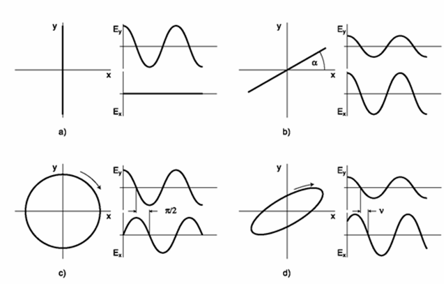
Fig. 2. a) linear polarization along the ordinate axis,
b) linear polarization (general case),
c) circular polarization, d) elliptic polarization. The image is from paper [4].
Figure 2 shows trajectories made by the tip of an electric field vector in a plane perpendicular to the ray.
Every electromagnetic wave is fully polarized in itself. A quasi-monochrome light ray, as a set of waves propagating in a single straight line and having the same wavelength, may be fully polarized, partially polarized, or unpolarized depending on the degree of correlation of oscillations of individual waves in the ray. If the oscillations are not correlated, the ray is unpolarized. If the degree of correlation is maximal, the ray is fully polarized and has one of the three above-mentioned types of polarization.
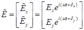
There exist several mathematical constructions (approaches) to describe and calculate the state of polarization: Jones vectors and matrices, Stokes vectors and Mueller matrices, coherence matrices and coherency modification matrices (for details, see [5, 6]). The Jones construction can be used only to describe fully polarized rays, whereas the other two constructions make it possible also to describe partially polarized rays. To meet the goals of this paper (that is, to estimate the degree of ray polarization), an approach based on coherence matrices (having a sufficient minimum of information) is convenient. Let us consider this approach in detail. The electric field of a fully polarized ray may be described by the Jones complex vector
 .
.
Here ![]() is the oscillation
frequency,
is the oscillation
frequency, ![]() and
and ![]() are the
initial oscillation phases,
are the
initial oscillation phases, ![]() and
and ![]() are the amplitudes of projections of electric
field oscillations onto two preselected vectors that are perpendicular to the wave
vector. The real electric field vector is
are the amplitudes of projections of electric
field oscillations onto two preselected vectors that are perpendicular to the wave
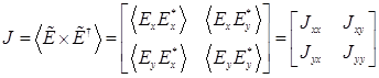
vector. The real electric field vector is ![]() . Then the
following matrix is called the coherence matrix [5, 6]:
. Then the
following matrix is called the coherence matrix [5, 6]:
 . (1)
. (1)
Here ![]() is mathematical
expectation,
is mathematical
expectation, ![]() is complex conjugation, and
is complex conjugation, and ![]() is transposition and complex conjugation. The
matrix and the basis for which it was calculated or measured (the ray and two vectors
that are perpendicular to the ray and to each other) determine the state of ray
polarization. The main diagonal elements of this matrix are real, and represent
the intensities of the
is transposition and complex conjugation. The
matrix and the basis for which it was calculated or measured (the ray and two vectors
that are perpendicular to the ray and to each other) determine the state of ray
polarization. The main diagonal elements of this matrix are real, and represent
the intensities of the ![]() - and
- and ![]() ‑
components of the electric vector. The ray intensity is equal to the trace of
the coherence matrix:
‑
components of the electric vector. The ray intensity is equal to the trace of
the coherence matrix:
![]() . (2)
. (2)
The extra-diagonal elements determine the degree of correlation of the electric field components. The following statements are valid:
1.
For natural (unpolarized)
light, the extra-diagonal elements of the coherence matrix are zero, and ![]() .
.
2. For fully polarized light, the determinant of the coherence matrix is zero.
3. The coherence matrix of rays propagating along a single straight line is equal to the sum of their coherence matrices.
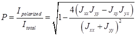
It should be noted that a partially polarized ray can be considered as the sum of two rays: a fully polarized ray and a fully unpolarized ray. The ratio between the intensity of the fully polarized part and the full intensity of the ray is called the degree of ray polarization. It is determined by the following relation [5]:
 . (2)
. (2)
That is, ![]() is equal to 1 for a fully
polarized ray and zero for natural light.
is equal to 1 for a fully
polarized ray and zero for natural light.
It makes sense to estimate the form of polarization of the fully polarized component. Let us introduce a concept of the degree of ellipticity of the fully polarized component of a ray as the ratio between the minor and major semiaxes of the ellipse made by the tip of the electric field vector. In this case circularly polarized light has a maximal degree of ellipticity of 1, and linearly polarized light, a minimal degree of ellipticity of 0. The degree of ellipticity can be calculated as follows [7]:
![]() , (4)
, (4)
where ![]() is the ellipse azimuth
(see below).
is the ellipse azimuth
(see below).
Another important parameter of the shape of an ellipse (in particular, that degenerating into a segment in the case of linear polarization) is azimuth, that is, the angle between the major semiaxis of the ellipse and the abscissa axis:
![]() . (5)
. (5)
The azimuth ranges in the interval ![]() . The lower and upper boundary values are
reached, for instance, at right and left circular polarization, respectively.
. The lower and upper boundary values are
reached, for instance, at right and left circular polarization, respectively.
Another important characteristic of the ellipse is its size. It is directly proportional to the ray intensity and, therefore, it is not reasonable to estimate the ellipse size separately. Such an image can be obtained in a standard way.
3. Visualization of polarization parameters in programs of optical design
The most popular traditional representation of fully or partially polarized rays in a text table format is not considered here. A set of initial data is constructed on the basis of a family of rays that have already been traced. The required picture is formed in a plane set by the user in the space of the scene (optical device). This image can be combined with another image obtained for this plane (see Fig. 3).
In [3], the User’s Manual, it is proposed to approximate unpolarized light on the basis of circular polarization. On the whole, the means of graphic representation of polarization are standard: ellipses, angles (azimuth), and eccentricities of ellipses.
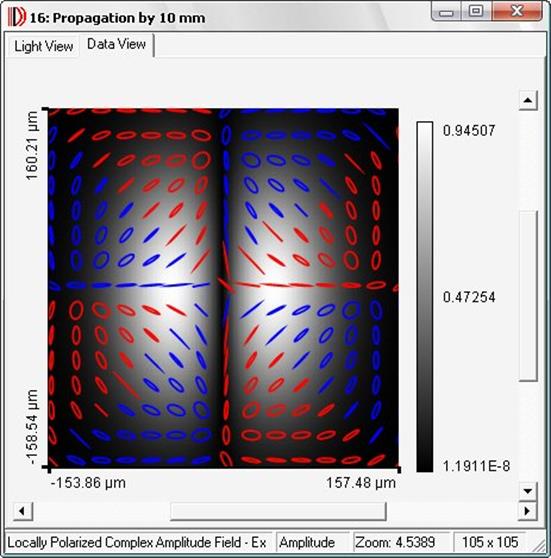
Fig. 3. An example of polarization image obtained
by program VirtualLab (see [3]).
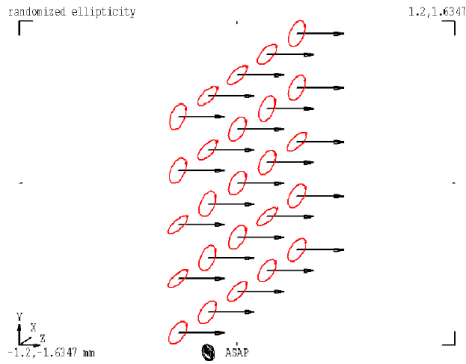
Fig. 4. An example of ellipticity image.
Arrows show ray directions.
Consider the most powerful tools for graphical analysis of polarization represented by program ASAP [2]. They are well-characterized by the series of screen images in Figs. 4 – 6.
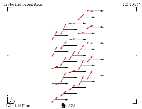
Fig. 5. An example of orientations image (azimuths).
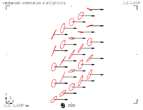
Fig. 6. Combined image of ellipticity and orientation.
In contrast to the other optical design programs, the ASAP versions of 2008 and later have a tool, the Poincaré sphere visualization tool (PSVT), for visual analysis of polarization for a family of calculated rays based on the Poincaré sphere (Fig. 7) (see [8]). ASAP allows calculations both with Jones vectors and Stokes vectors (parameters). In the latter case, the PSVT is used to analyze polarization.
Fig. 7. Stokes parameters shown on the Poincaré sphere (see [9]).
For each ray of the family being analyzed, we set a marker shape for the light wavelength and a color for the intensity. The sphere radius shows the degree of ray polarization (from 0 to 1). A typical screen image with PSVT is presented in Fig. 8.
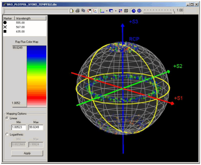
Fig. 8. Screen image with PSVT.
4. Proposed visualization method
The classical algorithms for photorealistic image rendering with ray tracing do not take into account the polarization property of rays. All calculations are usually based on geometrical optics, and the wave parameters of the ray (polarization and wave phase) are ignored. This can be explained by the fact that in scenes with diffuse objects the propagating light is not polarized, and light interference is observed only in some special scenes. Therefore, it does not make sense to calculate and take into account the wave properties of rays. This is an expensive and difficult task.
The wave properties of light may manifest themselves with translucent objects or metals added to a scene. In such cases the light changes its polarization state when it is reflected from them and passes through them. However, the change in light polarization in the general case of ray incidence on the surfaces of such objects is not very great and can be ignored. Again, the difference between the images calculated with and without allowance for polarization is noticeable [10].
If an anisotropic crystal (whose optical properties depend on the direction) is placed in a scene, the situation is quite different. The point is that such crystals are natural polarizers, i.e., the light passing through them is linearly polarized. With such polarization, due to the absence of axial symmetry of the ray electrical field, the interaction of the polarized light with objects greatly depends on the properties of these objects. Specifically, the light coming to another polarizer may be completely suppressed, or there may be no reflected rays when the light falls on a translucent isotropic object. Thus, the scenes containing anisotropic objects cannot be correctly calculated without allowance for light polarization.
On the whole, polarized light appears in a scene owing to [9]: 1) emission by a source; 2) anisotropy of the medium in which it propagates; 3) refraction and reflection at the boundary between two media.
In this paper, the presence of polarized rays in a scene and their polarization characteristics in scenes with above-mentioned polarization “sources” are studied in detail and visualized.
It should be noted that a jumpwise phase shift [11] affecting the interference in a scene can be observed under refraction at the boundary between two translucent media. However, this issue is not considered here.
The idea of visualizing polarized light distribution in a scene proposed in this paper is in modifying the classical camera used in ray tracing algorithms by making it “photograph” the needed parameters of incoming rays instead of their intensities (as it is done by the camera of standard renderers).
In this case, the modification is in the following. Each ray coming to the camera contains some information about the ray polarization, that is, the coherence matrix and the basis in which it was determined. A similar means can be constructed for other representations of polarization: Jones or Stokes vectors, Mueller matrices. To construct an image, the parameter being visualized must be calculated on the basis of this information and then transformed into the intensity of an image pixel to be recorded into a spectral image formed by the camera.
The algorithm of this transformation depends on the parameter being visualized. However, the general idea is to obtain intensity values that are parts of a standard spectrum. An advantage of this approach is that the image thus obtained can be transformed into an RGB-image by the standard CIE transform [12]. The resulting image will be called a map of some parameter, for instance, a polarization map of light in a scene.
Map of the degree of light polarization. The parameter ![]() varies
from 0 to 1. To obtain the intensity, it is simply multiplied by the spectrum
of a standard light source, CIE D65:
varies
from 0 to 1. To obtain the intensity, it is simply multiplied by the spectrum
of a standard light source, CIE D65:
![]() .
.
That is, for fully polarized light we obtain a CIE D65 spectrum (white), and for fully unpolarized light, a zero spectrum (black).
Map of the degree of ellipticity. The parameter ![]() varies
from 0 to 1. Also assume that the degree of ellipticity of unpolarized light is
zero:
varies
from 0 to 1. Also assume that the degree of ellipticity of unpolarized light is
zero:
![]() .
.
It is reasonable to calculate only monochrome images: if the spectrum is calculated for several wavelengths and recalculated into the RGB-color by the standard CIE transform, the color information thus obtained may become senseless, since the CIE transform uses only color information in the spectrum components.
For the experiments, a render (a program for polarized ray tracing) was used. For the calculations, a ray representation and a model of light interaction with crystals from [13] were used. As a photorealistic render it employs a method of backward recursive ray tracing, similarly to the Whitted algorithm [14]. That is, at the first pass a backward ray tracing tree is constructed, and at the second pass the illumination intensity is gathered only along the paths which terminate on light sources. This render was used to obtain test images in papers [13, 15]. Since only rays with known polarization enter the camera at the second pass, the render can display, in the camera picture plane, the required maps of the degree of polarization and ellipticity, in addition to the available basic mode – the intensity map.
Setting the necessary plane in a scene is setting the camera picture plane.
A virtual scene of a monocrystal and a square light source located under it was used for the numerical experiments. The source spectrum was determined by an RGB image transformed into spectral form by a method proposed in [12], and CIE D65 was used as the white spectrum.
A series of experiments has been performed to demonstrate the polarized light distribution in scenes with various light sources: 1) reflection and refraction of light on faces of a transparent isotropic object; 2) reflection and refraction of light on natural polarizers – anisotropic crystals; 3) scene illumination by a polarized light source.
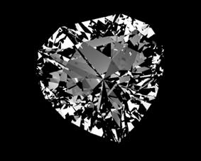
5.1. Optically isotropic transparent object
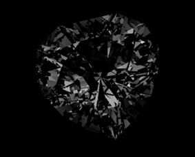
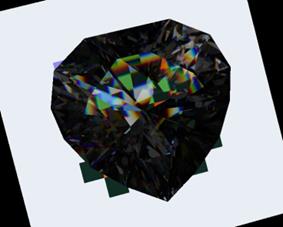
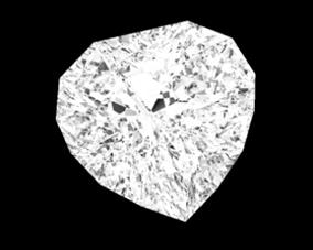
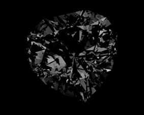
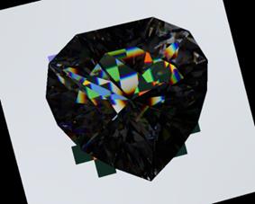
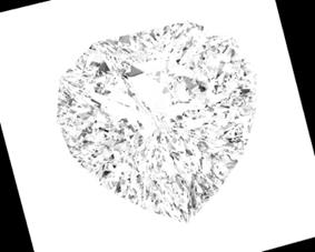
The object (a piece of transparent glass with a standard jewel facet) will be called a glass crystal (although glass does not have a crystalline lattice). One and the same scene has been calculated in four different modes. Figure 9 shows a full-color image calculated at 21 wavelengths uniformly distributed in the visible wave range from 380 to 780 nm. Figure 10 presents a monochrome image (580 nm). Figures 11 and 12 display polarization and ellipticity maps, respectively. The tracing depth for all of the above images is 9.
|
|
|
|
Fig. 9. Color image |
Fig. 10. Monochrome image (580 nm) |
|
|
|
|
|
|
|
Fig. 11. Polarization map (580 nm) |
Fig. 12. Ellipticity map (580 nm) |
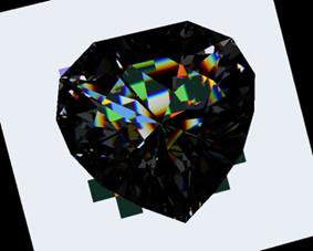

These images show a light source emitting unpolarized light (the light source is black in the polarization map) which may become partially polarized when passing through a crystal (Fig. 11) and partially become elliptic (Fig. 12). Elliptic polarization usually originates under full internal reflection or merging of partially and linearly polarized rays.
The spectrum ![]() of a
pixel in monochrome images for wavelength
of a
pixel in monochrome images for wavelength ![]() (Figs.
10, 14, and 18) is calculated as:
(Figs.
10, 14, and 18) is calculated as:
![]() ,
,
where ![]() is a calculated value,
is a calculated value,
![]() is CIE D65 spectrum, and
is CIE D65 spectrum, and ![]() is a spectrum value for the wavelength. As
a result, images look grey, not the color corresponding to the wavelength.
is a spectrum value for the wavelength. As
a result, images look grey, not the color corresponding to the wavelength.
5.2. Optically anisotropic transparent object
The situation with ellipticity and degree of light polarization in a scene changes if a glass crystal is replaced by an anisotropic crystal made from calcite. The result for an unpolarized light source is shown in Figs. 13–16. One can see from Fig. 16 that all light passing through the crystal becomes linearly polarized. No elliptically polarized light is present in the scene, since transparent anisotropic crystals are natural polarizers (only linearly polarized light can propagate in them).
|
|
|
|
Fig. 13. Color image
|
Fig. 14. Monochrome image (580 nm) |
|
|
|
|
Fig. 15. Polarization map (580 nm) |
Fig. 16. Ellipticity map (580 nm) |


Now the light source is changed for a linearly polarized source, that is, a crystal located on a liquid crystal monitor. For this, a virtual calcite plate is located above the source to pass the rays emitted by the source. Inside the plate, only one of the two rays formed at its boundary under refraction is considered in the algorithm. The optical axis of the plate was chosen so that the polarization plane of rays leaving the plate is parallel to the diagonal of the texture.
The result for a scene with a glass crystal is shown in Figs. 16–20. The monochrome and color images practically have not changed; the source is white in the polarization map, which implies its full polarization, and ellipticity still remained (although it is smaller than that in Fig. 12), although initially the illumination was linearly polarized.
|
|
|
|
Fig. 17. Color image |
Fig. 18. Monochrome image (580 nm) |
|
|
|
|
Fig. 19. Polarization map (580 nm) |
Fig. 20. Ellipticity map (580 nm) |


Figures 21–24 show results for a similar scene with an anisotropic calcite crystal.
Almost all light is fully polarized. In Figs. 15 and 23, the dark spots on the crystal image can be explained by the fact that part of the tracing rays does not reach the light source due to the limited depth of backward tracing. They are assumed to be unpolarized.
6. Debugging of renders and optical design programs
In the development of new algorithms and new software implementations of the existing algorithms (which is even more important), the effects of errors in the program code are often detected in the final target photorealistic image. In this paper, two maps with pixels containing exact information about polarization of the corresponding backward tracing path were added. In the full map, the observer often intuitively “feels” the image irregularities caused by a simple error in the code, for instance, an incorrect inequality of parameter values. The polarization visualization tools shown in Figs. 3–6 are based on a family of direct tracing paths that are finite in number (much less than the number of pixels) and show polarization at points which are small in number. These tools, which are based on stroke images, allow the designer to understand a general polarization pattern in a selected plane, but do not guarantee that a value at intermediate points may be obtained by simple “mental” interpolation. On the contrary, the maps can be obtained with different (larger) resolution. The PSVT tool (Fig. 8), in general, makes it possible to estimate the fraction of rays with some polarization parameters for a given family of paths (rays). The two visualization methods are not contradictory but are assumed to complement each other.
|
|
|
|
Fig. 21. Color image |
Fig. 22. Monochrome image (580 nm) |
|
|
|
|
|
|
|
Fig. 23. Polarization map (580 nm) |
Fig. 24. Ellipticity map (580 nm) |

As noted in the previous section, some paths constructed at the first stage of backward tracing from the camera may not reach illumination sources. Therefore, the corresponding map pixels may be underdetermined. To debug algorithms and programs one should not use geometrically complex objects (such as crystals presented in Figs. 9–24) but simpler scenes (such as a cube): a) consisting of objects made of complex optical materials; b) allowing the illumination sources to be reached in a small number of reflections/refractions; and c) based on well-known facts from optics. An example is an approach to creating scenes for testing a local model of light interaction with transparent objects [13]. It is described in [15] and has a permanently extended tests database [16].
In this paper, a method to visualize the polarized light distribution in a scene was proposed. This approach has proved to be informative, and it makes it possible to estimate the amount of polarized light, its distribution, and characteristics in a scene. The distribution is a function of some parameters, such as the degrees of polarization and ellipticity. In the ray tracing algorithm, the camera is modified to “photograph” any parameter of ray polarization (instead of the traditional ray parameter, i.e., intensity). Then it collects an image showing the distribution of the parameter values in the light coming from the scene.
The method developed above to graphically represent polarization for visual analysis may be of interest in itself. It can also help to debug algorithms of polarized ray rendering using well-known facts from optics and simple scenes with complex optical materials.
This visualization tool is based on a photorealistic render. Therefore, the method can be easily built into such programs as 3ds max® to support user plugins, for instance, as in [17] for structure visualization.
This work was partially supported by the Russian Foundation for Basic Research, project no. 12-07-00391 a.
[1] Brewster's angle. Available at http://ru.wikipedia.org/wiki/%D0%97%D0%B0%D0%BA%D0%BE%D0%BD_%D0%91%D1%80%D1%8E%D1%81%D1%82%D0%B5%D1%80%D0%B0.
[2] Optical software ASAP. Available at: http://www.breault.com/software/asap.php.
[3] LightTrans VirtualLab User’s Manual, August 2013. Available at: http://www.lighttrans.com/documents.html?&no_cache=1&tx_abdownloads_pi1%5Baction%5D=getviewclickeddownload&tx_abdownloads_pi1%5Buid%5D=1439&tx_abdownloads_pi1%5Bcid%5D=1796/.
[4] Devlin K., Chalmers A., Wilkie A., Purgathofer W. STAR: Tone reproduction and physically based spectral rendering. Eurographics 2002. pp. 101–123.
[5] Born M., Wolf E. Principles of optics: electromagnetic theory of propagation, interference and diffraction of light. Cambridge: Cambridge University Press, 1980.
[6] Tannenbaum D.C., Tannenbaum P., Wozny M.J. Polarization and birefringency considerations in rendering. Comp. Graphics (SIGGRAPH'94 Proceedings), ACM Press, pp. 221–222.
[7] Shurcliff W.A. Polarized light: production and use. Harvard University Press, 1962.
[8] Poincaré sphere visualization tool. Available at: http://www.breault.com/resources/kbasePDF/bro4310_Polarization.pdf.
[9] Polarization (waves). http://en.wikipedia.org/wiki/Polarization_(waves).
[10] Debelov V.A., Kozlov D.S., Sattarov M.A.Rendering of monocrystals with polarized ray. Proceedings of 6th International Workshop on Virtual Environment on PC Cluster, VEonPC'2006, Protvino-Altai. Protvino, pp. 15–22 (in Russian).
[11] Fedorov F.I., Filippov V.V. Reflection and refraction of light by transparent crystals. Minsk: “Nauka i Tekhnika,. 1976 (in Russian).
[12] Glassner A.S. How to derive a spectrum from an rgb triplet. IEEE Comput. Graph. Appl, vol. 9, 1989, pp. 95–99.
[13] Debelov V.A., Kozlov D.S. A Local Model of Light Interaction with Transparent Crystalline Media. IEEE Ttransactions on visualization and computer graphics, vol. 19, № 8, 2013, pp. 1274-1287.
[14] Whitted T. An improved illumination model for shaded display. Commun. ACM, vol. 23, № 6, pp. 343–349, 1980.
[15] Debelov V. A., Kozlov D. S. Rendering of translucent objects, verification and validation of algorithms. Proceedings of the 20th International Conference in Central Europe on Computer Graphics, Visualization and Computer Vision, Pilsen, Czech Republic, Jun. 2012. Available at: http://wscg.zcu.cz/wscg2012/CDROM/WSCG-2012-CD-ROM.zip.
[16] Pre-repository of tests' descriptions. Available: http://oapmg.sscc.ru/temp_crystal_tests/.
[17] Strikhanov M.N., Degtyarenko N.N., Pilyugin V.V., et al. Computer visualization of nanostructures experience at NRNU "MEPhI". Scientific Visualization, vol. 1, № 1, 2009, pp. 1–18. Available at: http://sv-journal.com/2009-1/01.php?lang=en.