Abstract
It is proposed an integrated solution for animation, interaction with dynamic objects and visualization of large grasslands. We use instancing for real-time visualization. For that, a new method for physics animation was developed which does not require saving generalized velocities and moves for each grass blade.
Keywords: Real-time, Animation, Collision, Rendering, Grass.
1. PREVIOUS WORKS
There are three methods for the grass visualization: geometry-based, image-based и volume-based. According to the first method, each grass blade is defined with a set of triangles. The set of the blades shapes a rectangle block. The block is visualized repeatedly in order to cover all the grass area. To speed up visualization, instancing technique is used. This geometry-based method was used in [3], [8] and [10] papers. The problem of this method is visualization of hundreds of millions of triangles. For cutting down this number, it was proposed in [3] to reduce the number of triangles in the blade if the latter is far from camera.
Image-based method distinguishes from the described above with only one feature: the set of blades in the block is replaced with the set of billboards with the texture containing alpha channel; a set of blades is drawn on it. This method was used in [2], [5], [6] and [9] papers. Volume-based method was applied in [7, 8]. Based on these approaches, it is difficult to get high quality of visualization close to the camera.
In order to increase visual realism, all mentioned methods are accompanied by the grass animation. In all cases it is used simplified model: the movements are proportional to the wind force and directed along its velocity vector.
Grass interaction with dynamic objects during the animation process was considered in [12] and [6]. In the first of these papers real interaction was substituted with use of a special texture – the footprint of the moving object. In the second one the object interacted with billboards that simulated the grass.
2. VISUALIZATION
2.1. Basic principles
We use geometry-based approach. According to it, similar to [8] rectangular blocks are created; each of them consists of a set of separate blades. These blocks are visualized on the terrain surface. A set of grass blocks makes up the rectangular grid which is mapped onto terrain such way that the central cell of the grid appears just under camera. When the camera moves on the adjacent grid cell the whole grid moves on the grid cell size.
The grass covering is visualized by multiple repetition of the single grass block according to instancing method with correcting position and shape of each grass blade in compliance with the terrain height and wind force in the given point.
Some part of the grass blocks is not included in instancing. These are the blocks in which interaction of grass blades with other dynamic objects is possible, as well as such interaction has occurred. For these blocks wind simulation calculations use numerical methods that require storing current positions and velocities of the grass blade tops, which excludes instancing. Let us denote these blocks “patches”. They are visualized as objects containing a set of grass blades.
The grass block is a square containing N=n*n blades. In terms of DirectX10 each blade is a point containing four vertices and the normal determining rotation angle of the blade plane and the angle to the terrain surface, as well as geometry (length and height) and physics (mass and rigidity) characteristics. This data and the wind force vector are input data for the vertex shader to calculate the current location of the vertices and values of normals in them. Then, the geometry shader builds a cubic spline, that determines the blade triangles, number of which depends on the distance between the blade and the camera.
2.2. Levels of detail and smooth transition between them
We introduce three discrete levels of detail for the grass blocks, as well as possibility of smooth changing of detail within a level. To provide the possibility of smooth changing of detail, a weight coefficient is assigned to each blade in the block. When visualizing, the blade is discarded, if the following condition is valid:
2.3. Lighting calculation
For a single directional light source applied to a point of the surface of a blade, the radiance I is:
![]()
Where ![]() is the material ambient color,
is the material ambient color, ![]() - the diffuse reflectance factor of the blade material,
- the diffuse reflectance factor of the blade material, ![]() - the intensity of the ambient light,
- the intensity of the ambient light, ![]() - the normal to the grass blade surface,
- the normal to the grass blade surface, ![]() - the light direction,
- the light direction, ![]() – the factor to account for the color change of light traversing the
grass blade fibers,
– the factor to account for the color change of light traversing the
grass blade fibers, ![]() - the intensity of the light
source.
- the intensity of the light
source.
Because the grass blades shade each other, intensities of diffused and direct sun light should be considered as functions of distances between the blade base and top. We use the following dependences:
![]()
![]()
where ![]() ,
, ![]() - intensities on the blade top,
- intensities on the blade top, ![]() - intensity on the base, l – normalized distance from the base to
the top.
- intensity on the base, l – normalized distance from the base to
the top.
For Frenel effect simulation while calculating light
for the blades on contour terrain areas we increase the calculated intensity
value ![]() by
by ![]() value:
value:
![]()
where ![]() is the specular reflectance
factor of the grass blade material,
is the specular reflectance
factor of the grass blade material, ![]() - normal to the terrain surface
and
- normal to the terrain surface
and ![]() - vector of direction to the
camera.
- vector of direction to the
camera.
3. ANIMATION
3.1. Inertial animation model
Let us represent the blade model with the chain of n
linear segments, connected each to other with joints in which there are
spherical springs (Fig. 1). We will denote the rigidity of these springs as ![]() where i – number of the joint.
where i – number of the joint.
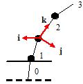
Fig. 1. The blade model for n = 4
The coordinate system is assigned to each segment as shown on Fig. 1. The segments and joints are enumerated bottom-up. Zero segment is dummy and determines initial rotation and tilt angles of the blade when planting. Ground level is on the height of lower end of the first segment (joint 1).
Let the following external forces ![]() are applied to the segment centers – the forces, which
are the sum of the wind force and the segment gravity (Fig. 2).
are applied to the segment centers – the forces, which
are the sum of the wind force and the segment gravity (Fig. 2).
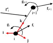
Fig. 2 Forces and moments applied to the segment
Let us write movement equation for i-segment in its coordinate system:

Here:J– inertia
tensor, ![]() - vector of angle velocity of
i-segment,
- vector of angle velocity of
i-segment, ![]() – vector determining rotation increment of the coordinate system of
i-segment, relatively to the coordinate system of (i – 1) segment ,
– vector determining rotation increment of the coordinate system of
i-segment, relatively to the coordinate system of (i – 1) segment , ![]() - the moment because of spring in i-joint,
- the moment because of spring in i-joint, ![]() – matrix converting vectors from the coordinate system of i-segment to the
coordinate system of (i-1)-segment (when i=0 – to the world coordinate system),
– matrix converting vectors from the coordinate system of i-segment to the
coordinate system of (i-1)-segment (when i=0 – to the world coordinate system), ![]() - matrix, converting vectors from the world coordinate system to the coordinate
system of i-segment,
- matrix, converting vectors from the world coordinate system to the coordinate
system of i-segment, ![]() - acceleration at the end of i-segment, l= (0,0,l)’, where l – a half of the segment length, m – mass of
the segment.
- acceleration at the end of i-segment, l= (0,0,l)’, where l – a half of the segment length, m – mass of
the segment.
For integration of the system we can be used Featherstone algorithm [11]. However, the computational complexity of this integration is too expensive to calculate the animation of several thousand blades of grass in real time.
We can simplify this system, if assume that: angle velocities are small and impact of higher segments on lower is much less, than reverse. The first assumption allows us to discard members containing squares of angular velocities, and the second – to refuse of the second pass in Featherstone algorithm. As a result, we come to the following simplified algorithm:
T0=R0
for (i=1; i<n; i++) {
![]()
![]()
![]()
![]()
![]()
}
where M(ψ) – matrix of rotation around the vector ψ the value | ψ |, V - inverse transform to get rotation vector.
As our experiments showed, this algorithm keeps good visual illusion of animated grass blades.
3.2. Animation of wind force and direction
Similarly to [1] we use the cyclic Perlin noise
texture. Wind animation is done by summing up (with various scales ![]() ) three such textures moving with
) three such textures moving with ![]() velocities (i=1, 2, 3). Resulting wind speed vector
velocities (i=1, 2, 3). Resulting wind speed vector ![]() in the texel with u coordinates is calculated with the
formula:
in the texel with u coordinates is calculated with the
formula:
![]()
where ![]() - scale coefficients, t – time,
- scale coefficients, t – time,
While calculating wind force for each blade segment, we consider velocity of the segment:
![]()
Here ![]() - coefficient depending on the blade width, vi- velocity of the segment center,
- coefficient depending on the blade width, vi- velocity of the segment center, ![]() - a constant depending on the grass type (for example,
- a constant depending on the grass type (for example, ![]() =4/3 for sedge). vi value is calculated depending on
=4/3 for sedge). vi value is calculated depending on ![]() (velocity of the top of previous
segment) according to formula:
(velocity of the top of previous
segment) according to formula:
![]()
Velocities of the segment tops are found from recurrent relations:

3.3. Virtually-inertial animation model
This model provides results close to that for inertial model, but doesn’t require storing current values of angle velocities and general displacements for each grass blade, which allows us to use instancing when rendering.
The idea of the virtually-inertial model is in carrying over inertial component from calculation of the blade shape to calculation of the wind force for this blade. That may be done if we put into centers of wind force texels vertical virtual blades and calculate their shape with inertial model. Afterwards we calculate the moments that must be applied to blades segments in order to get the same shape of static equilibrium:
![]()
where G – gravity (here, as well as in the previous paragraph do not consider the effect of the upper segment to lower). These moments are stored in the virtual wind texture that is used for the grass blade animation when rendering with instancing, instead of the actual wind forces.
Note that the blades covered by one texel of virtual wind texture should be animated differently in spite of they are affected by the same virtual wind. This is because they have various angles when planting, so weight force impact is diverse.
To do so, we calculate the shape of a blade of grass so that the condition of static equilibrium under the action of the virtual wind and gravity, taking into account the slope of grass with seating. The equation of static equilibrium for the i-th segment is as follows:
![]()
With known matrix ![]() this
equation can be solved by simple iteration. As our experiments showed,
three iterations are enough for coinciding visual results.
this
equation can be solved by simple iteration. As our experiments showed,
three iterations are enough for coinciding visual results.
Thus, we arrive at the following algorithm for determining the shape of a blade of grass:
![]()
for (i=1; i<n; i++){
![]()
![]()
![]()
}
Here, the matrix T0 defined angle of seating.
3.4. Animation algorithm considering interaction with other dynamic objects
For simulation of grass interaction with dynamic objects, as mentioned in section 2.1, patches instead of blocks are used. Blade data structures in patches contain fields for current generalized velocities and moves, which allows us to use an inertial model. Nevertheless, we continue to use virtual-inertial model until the blade interacts with an object. At this moment the blade segments are bent so that exclude intersections with the object and its generalized velocities are set to zero. Later such blade is calculated with inertial model.
This approach allows us to use an expensive inertial model only for relatively small number (around a thousand) of grass blades.
Note that use of different models for close located blades doesn’t lead to visual artifacts due to proximity of these models.
4. RESULTS
Visual results of our program are presented on Fig. 3, 4 screen shots. Fig. 3 shows grass animation with a wind and Fig. 4 shows the result of grass interaction with a dynamic object without and with the wind
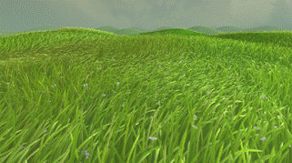
Fig. 3. Grass animation with a wind
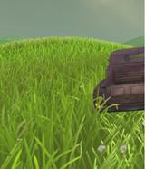
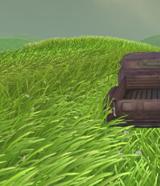
Fig. 4. Grass interaction with a dynamic object without and with the wind.
Video material can be can be found here:
http://dl.dropbox.com/u/28177387/GrassCar.avi
http://dl.dropbox.com/u/28177387/GrassPlain.avi
The grass field covers the
square with the side of
It is evident from the Table 1 that about 90% program time is spent for visualization and only 10% - for processing interaction with dynamic object and calculating blade shapes under wind. That proves high efficiency of the developed algorithms and possibility of their use in real-time programs.
PC configuration |
A |
B |
C |
FPS |
FPS |
FPS |
|
Intel Pentium D CPU 3GHz ATI ASUS EAH5450 |
28 |
26 |
24 |
Intel Core 2 Duo e8500 Nvidia GeForce 9600 GT |
60 |
57 |
54 |
Intel Core 2 Duo e8500 ATI Radeon HD 6870 |
180 |
165 |
150 |
Table. 1. The program performance
5. ACKNOWLEDGEMENTS
The work was funded by Intel A/O (Agreement #NN/R&D/66/2010).
6. REFERENCES
1. Alexandre Meyer, Fabrice Neyret. “Interactive Volumetric Textures”. Eurographics Rendering Workshop, 1998.
2. Anu Kalra. “Rendering Grass with Instancing in DirectX* 10, 2009.“. Available at: http://isdlibrary.intel-dispatch.com/vc/2325/rendering_grass_32509.pdf
3. By Changbo Wang, Zhangye Wang, Qi Zhou, Chengfang Song, Yu Guan and Qunsheng Peng. “Dynamic modeling and rendering of grass wagging in wind”. Comp. Anim. Virtual Worlds, pp.377–389, 2005
4. “Cloth Simulation”. NVIDIA White Paper, sdkfeedback@nvidia.com, 2007
5. David Whtley. “Toward photorealism in virtul botany”. GPU Gems 2, pp. 7-25, 2005
6. J. Orthmann, C. Rezk-Salama, A. Kolb. “GPU-based Responsive Grass”. In Journal of WSCG, 17, pages 65-72, 2009.
7. Ralf Habel, Michael Wimmer, Stefan Jeschke. “Instant Animated Grass”, 2009. Available at: http://www.cg.tuwien.ac.at/research/publications/2007/Habel_2007_IAG/Habel_2007_IAG-Preprint.pdf
8. Kevin Boulanger, Sumanta Pattanaik, Kadi Bouatouch. “Rendering Grass in Real Time with Dynamic Lighting”. IEEE Computer Graphics & Applications, vol. 29(1), pp. 32-41, 2009.
9. Kurt Pelzer, Piranha Bytes. “Rendering Countless Blades of Waving Grass”. GPU Gems. Chapter 7, 2004.
10. Perbet F, Cani M-P. “Animating prairies in real-time”. In Proc. the symposium on Interactive 3D graphics, pp. 103-110, 2001.
11. Roy Featherstone, D. Orin “Robot dynamics: equations and algorithms”. Proceedings 2000 ICRA Millennium Conference IEEE International Conference on Robotics and Automation Symposia Proceedings Cat No00CH37065 (2000)
12. Sylvain Guerraz, Frank Perbet, David Raulo,
Franc¸ois Faure,