USAGE OF LOCAL ESTIMATION AND OBJECT SPECTRAL REPRESENTATION AT THE SOLUTION OF GLOBAL ILLUMINATION EQUATION
V. Budak, V. Zheltov, T.Kalakutsky
Moscow Power Engineering
Institute (TU), Light Engineering Department,
budakvp@mpei.ru, zheltov@list.ru, kalakutskytk@mpeil.ru
Contents
3.Accuracy evaluation of local estimation.
5.Spectral representation of objects.
7.Realization of local estimaion method and rendering objects represented by spherical harmonics.
The solution
simulation of the global illumination equation by the local estimation of the
Keywords: Global Illumination, Monte Carlo, Local estimation.
3D scene simulation is inherently the calculation of object luminance on the basis of the solution of the global illumination equation, which is an integral equation of the second order [1]:
where ![]() is the luminance at
the point r in the direction
is the luminance at
the point r in the direction ![]() ,
, ![]() is bidirectional
scattering distribution function (reflection or transmittance), L0 is the luminance of the
direct radiation straight from sources.
is bidirectional
scattering distribution function (reflection or transmittance), L0 is the luminance of the
direct radiation straight from sources.
The equation has no analytical solution at an arbitrary
law of reflection, so the methods of numerical simulation are used. The
The reverse ray tracing suffers from basic defects connected with that the sizes of light sources as a rule are sufficiently small and the expectancy of hitting in the source is very low.
In case of the direct simulation the scene is divided into elements, in which the photon hits are calculated. As a result the illumination map is created. This approach is connected with the complications of mesh generation and the excessive consumption of memory.
The finite element method, which is called in the global illumination theory as a radiosity [3], is used for the solution of equation on the basis of diffuse reflection approximation. In this case the equation could be rewritten as [3]
where M(r) is the luminosity of the surface in
point r, M0(r) is the
luminosity of the surface in point r straightforward from sources, ![]() is the visibility
function of element
is the visibility
function of element ![]() from point
from point ![]() ,
,  is the infinitesimal
form-factor.
is the infinitesimal
form-factor.
In our paper we propose to use the local estimation of the Monte-Carlo method, which are well-known in the optics of atmosphere at the solution of radiative transfer equation [2, 4]. Rendering 3D objects represented by the spherical harmonics spectrum is analyzed in the paper.
Equation is not convenient for the statistic
simulation, as the unknown function is under the integral in the point r′,
but it is determined in the point r.
In addition to that the variables r′ and ![]() are not independent, and
combined by the relation
are not independent, and
combined by the relation
 .
.
Accordingly we can write down the equation in the following form
![]()
This expression
contains the δ-function impeded the simulation by the local estimation of
the
![]() takes a form
takes a form
where k(r,r′) is the kernel of , Qn is the weight of Markov chain, and M is the mean operator by the different random ray trajectories.
Markov chain in
this case represents the sample of random ray trajectory, which is created
using ![]() as an initial
probability and k(r,r′) as a transition
probability [2, 4]. From every knots of this random ray trajectory rʹ, which coincide with the
intersection points of ray with object surfaces, is calculated the contribution
in the illumination in the given point r by the term k(r,r′) in expression .
as an initial
probability and k(r,r′) as a transition
probability [2, 4]. From every knots of this random ray trajectory rʹ, which coincide with the
intersection points of ray with object surfaces, is calculated the contribution
in the illumination in the given point r by the term k(r,r′) in expression .
Of course all the
probability distribution must satisfy to the normalizing condition. The distinctions
of ![]() and k(r,r′) from this
condition generate the statistical weights Qn.
For example, in case of the diffuse reflection it is equal to the surface
reflectivity.
and k(r,r′) from this
condition generate the statistical weights Qn.
For example, in case of the diffuse reflection it is equal to the surface
reflectivity.
The expression was called the local estimation of the
Let’s note that as opposed to the classical ray tracing the local estimation allows estimating in several points at once by one statistical sampling ray that sufficiently accelerates the convergence of calculations.
The accuracy estimation of algorithm is possible on the basis of comparison with other known methods or with exact analytical solution of the equation for some special situation. It is known two exact analytical solution of the global illumination equation: for the Ulbricht sphere and for so called Sobolev problem [9]. In case of the Ulbricht sphere we have the uniform distribution of the luminosity over sphere that makes this case ineffective for the accuracy estimation. In the Sobolev problem we solve the for the luminosity distribution in case of the illumination of two parallel diffuse reflecting planes by the point isotropic source located between these planes. In this case the equation is transformed to the set of two integral equations (for the first plane):
where Ei(r) is the illuminance of i-th plane (i=1,2), i is the reflection coefficient of i-th plane, hi is the distance from the source to the i-th plane. We assume the source intensity equal to 1 and h1+h2=1.
For the solution of the equation set let’s execute the Fourier transformation of each equation that results in the set of linear algebraic equations. After the solution of the obtained equation set and inverse Fourier transformation we get the following expression:
![]()
where K1(k) is the modified Bessel function of second kind, J0(kr) is the Bessel function of first kind.
In Figure 1 we can see the numerical comparison of the luminosity distribution calculation by the local estimation method and the expression .
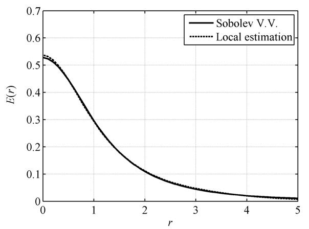
Figure 1. Illuminance distribution in case of the Sobolev problem:
h1 = h2 = 0.5, and reflection coefficients ρ1 = ρ2 = 0.5.
In this case it was used 2000 rays at the calculation by the local estimation method, and the running time was less than 1 second for the computer AMD Athlon 64 X2 5200.
We realized also the solution of the Sobolev problem by the radiosity, and compared it with the local estimation: the local estimation exceeds the radiosity in computation speed at 80-90 times for the equal calculation accuracy.
The equation of global illumination can be represented in the operator form
![]() .
.
The solution of this equation is represented in the form of the Neumann series that allows conducting following transformations
![]()
![]() ,
,
that results in normal a form

The local estimation corresponding expression can be called as double local estimation [2, 4] and takes the following view
![]() ,
,
where
In the expression the δ-function is eliminated as a
result of integration, and independent variables ![]() correspond to the
geometry of ray propagation [4].
correspond to the
geometry of ray propagation [4].
Thereby the double local estimation allows modeling the global illumination equation solution and calculating straight the luminance of incident radiation in the given point for the reflectance of orders higher than the first taking into account an arbitrary reflectance law. The first order can be calculated directly.
We do not know currently any software, which is capable to calculate the luminance directly. Thereby the double local estimation for the first time in light engineering and computer graphics allows computing the spatial-angular distribution of luminance in the given point of space.
Standard representation for the 3D objects is the mesh representation, in which objects are described by the set of vertices connected into faces. Such representation is universal and allows describing any object. However it is not capable to reproduce exactly many objects, and in case of the essential error influence on the result the solid modeling can be applied, when objects are described analytically. SolidWorks and TracePro are the most known programs using the similar approach.
One of the challenging directions of the 3D object representation is the spectral representation on the basis of spherical harmonics [5] that is the object surface representation by the series of spherical harmonics. In the sequel we will use the term “spectral representation” for short. Such object representation gives a possibility of the reproduction quality control. So objects located far from a camera can be reproduced with low quality. In terms of photometry the essential advantage of this approach is the continuous representation of surface normals without any approximation. Let’s analyze the mathematical techniques underlying the method of spectral representation.
The spherical
harmonic ![]() is the special
function defined on the unit sphere
is the special
function defined on the unit sphere
![]()
where θ is the zenith angle [0 π], φ is the azimuth angle [0 2π], Akm, Bkm are some coefficients, ![]() is the associated
Legendre polynomials. The major property of spherical harmonics is their orthogonality:
is the associated
Legendre polynomials. The major property of spherical harmonics is their orthogonality:
 ,
,
where δ is the delta Kronecker symbol.
Owing to this property any twice continuously differentiable function can be expanded into uniformly and absolutely convergent series of spherical harmonics [6]
![]() ,
,
where Akm, Bkm are the Fourier coefficients determined by formulae
 ,
,
 ,
,
and ![]() is the norm determined
by the expressions
is the norm determined
by the expressions

The calculation of factorial is the substantial complication by the expansion. As a result it is the essential difference of coefficients resulting in the extra miscalculation. At the expansions of spherical harmonics it is more convenient to use the Schmidt polynomial determined as
 .
.
It is not difficult to see that at the Schmidt polynomial expansion there is no necessity to calculate the factorials for the norm and that essentially improved productivity of calculations.
Therefore, any object defined unambiguously on radius from some point can be expanded by spherical harmonics.
At the global illumination equation solution by the local estimation method it is necessary to calculate surface normal and to determine the cross point of ray with an object. In case of the mesh object representation this problem is not difficult, but in case of the spectral representation it becomes a hard one. We analyze the determination of normal to the given point of object defined in the basis of spherical harmonics.
The normal in the
point ![]() on the surface defined
in the spherical coordinate system is equal the value of its gradient in this
point
on the surface defined
in the spherical coordinate system is equal the value of its gradient in this
point
For the function described the surface in the spherical coordinate system we can write down the expression
![]() .
.
Let’s find partial derivatives in accordance with the equation . The derivative with respect to r
The derivative with respect to φ

The derivative with respect to θ

Consequently, it is necessary to calculate the derivative of the Schmidt polynomial. It is known the recurrent relation for the Legendre polynomial [7]

that taking into account the relation between the Schmidt and Legendre polynomial [7]
![]() ,
,
allows to receive after some transformations the final expression
![]()
It is necessary to analyze separately the case m=0. In this case taking into account a number of the relations [8] it is not difficult to result in
![]() .
.
Using the derived
gradient in the local spherical coordinate system ![]() it is necessary to
represent it in the world Cartesian coordinate system. Taking into account some
known relations ones can get the final expression for the normal to object
surface represented by spherical coordinates
it is necessary to
represent it in the world Cartesian coordinate system. Taking into account some
known relations ones can get the final expression for the normal to object
surface represented by spherical coordinates

 .
.
The search of the point of ray intersection with the object represented by the spherical harmonics is also a nontrivial task. Let’s consider the object represented relative to the origin of the Cartesian coordinate system and the ray
![]() .
.
The cosine of angle θ of the point of ray intersection with the surface can be written as
For the vector ρ we have accordingly
![]() .
.
The cosine and sine of angle φ have the form
 ,
,
Therefore we get the dependence of angles θ and φ on one variable ξ. The equality takes place in the point of intersection
Solving the equation relatively the parameter ξ we can find all the point of ray intersection with the object surface. In case of the global illumination equation solution for scene rendering we are interested only by the first intersection with the object. It can be found both the standard procedures, for example the bisection method, and more complex and fast algorithms.
We implemented the algorithms of the local and double local estimations with 3D object representation in the basis of spherical harmonics. In Figure 2 we see rendering of the simple 3D scene. It is the room represented by the mesh with one column and one omni light source. The head of man in the scene is represented by the surface harmonics. The initial mesh contains 32 654 edges. In Figure 1 it was used N = 32 spherical harmonics to play the head. In this case the rendering time increased by 40% in comparison with the visualization of the mesh, but the amount of stored information decreased in more than 1,000 times.
Figure 2. 3D scene rendering by the local estimation method.
The local
estimation method of the
The usage of the object spectral representation on the basis of spherical harmonics is the successful approach for the description of some class objects that allow reducing significantly the information content, which is necessary for the adequate reproduction. The possibility of continuous normal retrieval with the control accuracy in aggregate with the local estimation method is an important approach in the 3D scene rendering and its photometric investigation. The continuous restoring of normals has the special importance in case of luminance angular distribution calculations, where the wrong normal approximating results in considerable degradation of calculation accuracy.
1. Budak V.P. Visualization of luminance distribution in 3D scene. – M.: MPEI, 2000. (in Russian)
2. Monte-Carlo
Methods in Atmospheric Optics. G.I.Marchuk, ed. –
3. Foley J.D., van Dam A., Feiner S.K., Hughes J.F. Computer graphics: principles and practice. Addison-Wesley, 1997.
4. Ermakov S.M., Mikhailov G.A. Course of statistical modeling. - M.: Nauka, 1976. (in Russian)
5. Mousa M., Chaine R., Akkouche S. Frequency-Based Representation of 3D Models using Spherical Harmonics // The 14-th International Conference in Central Europe on Computer Graphics, Visualization and Computer Vision "WSCG'2006", Plzen, Czech Republic, January 31 – February 2, 2006. Full Papers Proceedings, p.193-200
6. Tikhonov A.N., Samarsky A.A. Equations of Mathematical Physics. – M.: Nauka, 1976. (in Russian)
7. Vilenkin N.Ya. Special functions and
the theory of group representations. Translated from the Russian by V.N. Singh.
Translations of Mathematical Monographs, Vol. 22 American Mathematical Society,
8. Mishchenko M.I., Travis L.D., Lacis A.A.
Scattering, Absorption, and Emission of Light by Small Particles. -
9. Sobolev V.V. Point light source between parallel planes. Doklady of the Academy
of
 ,
,  .
.  ,
,  ,
, 
 .
.  .
.