R2 or R3 be the signed distance function to an oriented closed
surface M. The function d is the vanishing viscosity solution of the Eikonal
equation [23, 21, 19]:
R2 or R3 be the signed distance function to an oriented closed
surface M. The function d is the vanishing viscosity solution of the Eikonal
equation [23, 21, 19]:
fayolle@u-aizu.ac.jp, apasko@bournemouth.ac.uk
Contents
We present in this paper methods to compute the signed Euclidean distance to surfaces obtained by the intersection (respectively union or difference) of two solids (in two or three dimensions). These implementations can replace min/max or R-functions traditionally used to model set operations used with implicit surfaces.
Keywords: shape and solid modeling, constructive modeling.
In shape modeling, a solid can be defined by the sign of a continuous function: the set {p : f(p) ≥ 0} defines the interior and the boundary and the set {p : f(p) < 0} the exterior (the so called implicit surfaces or F-Rep, see [3], [11] and the references therein). The particular case where f is the signed Euclidean distance to the boundary of the solid is of special interest. Distance based models are extremely useful in many applications such as: constant-radius offsetting and blending operations [16], surface metamorphosis and smoothing [13], object reconstruction from a set of cross-sections [9], rendering with sphere tracing [5], generation of skeletal shape representation [24], heterogeneous object modeling [2] and others. We present in this paper methods for calculating the signed Euclidean distance from a point to the surface of a solid constructed by applying set-theoretic operations (union, intersection, difference) to primitives defined by distance functions. That is: if d1 and d2 represent the distances to the surfaces of two primitives S1 and S2, we present an algorithm for calculating the distance d to the surface of the union (respectively intersection, difference) of S1 and S2.
Let d(p), p R2 or R3 be the signed distance function to an oriented closed
surface M. The function d is the vanishing viscosity solution of the Eikonal
equation [23, 21, 19]:
 |
(1) |
where ∥.∥2 – the Euclidean norm.
Let c be the closest point to p in the surface M, the signed distance is then ϵ∥p - c∥2, where ϵ = -1 if p is outside the solid delimited by the surface M, 1 otherwise. If the surface is smooth, then p - c is orthogonal to the surface. The signed Euclidean distance function is continuous but not everywhere differentiable.
Expressions for the distance function to most of the typical surfaces of a CSG system (sphere, cylinder, cone) are known analytically [5] and distance to general quadrics and ellipsoids can be computed by a numerical procedure [6].
In general, if the surface M is available as an oriented point-set or a mesh of polygons, it is possible to solve the Eikonal equation (Eq. (1)) on a finite grid. There exist various numerical algorithms such as the fast marching method [19], the fast sweeping method [21, 23], or the characteristics / scan conversion algorithm [10]. Algorithms exploiting the GPU have also been designed in order to compute efficiently the Euclidean distance function on a grid [7, 20]. Once a grid is obtained, with the signed Euclidean distance to M sampled at each grid node, it is possible to apply spline interpolation or approximation to get a function approximating the distance [15].
In constructive geometry, complex solids are built by applying successively set operations (union, intersection, difference) to primitives. For solids described using real valued functions, like in implicit surfaces or F-Rep modeling systems, expressions for these operations have been proposed by Sabin [18], Ricci [14] and Rvachev [17].
Sabin [18] and Ricci [14], independently proposed the use of the functions min and max to implement the intersection and union of implicit surfaces. If d1 and d2 are the functions defining two solids, then the union is defined by the function max(d1,d2) and the intersection by min(d1,d2) (the difference operation is obtained by min(d1,-d2), i.e. by replacing d2 by -d2). Rvachev proposed the R-functions [17]:
d1 ∨αd2 =  (d1 + d2 + (d1 + d2 +  ) ) |
(2) | |
d1 ∧αd2 =  (d1 + d2 - (d1 + d2 - ) ) |
(3) | |
| d1 \αd2 = d1 ∧α(-d2) | (4) |
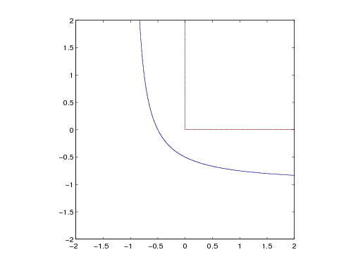
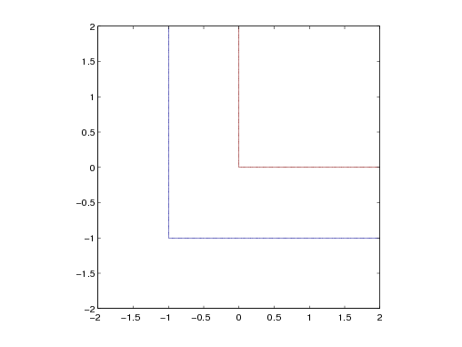
Neither the scalar field obtained by using min/max nor the R-functions correspond to the Euclidean distance to the surface of the constructed solid. This is illustrated in Fig. 1, where the approximate distance field to the surface made by the intersection of the halfspaces: x ≥ 0 and y ≥ 0 is computed using an R-function (left) and min (right). The red curve corresponds to the solid boundary (i.e. corresponds to the distance 0) and the blue curve to the set of points at a value of -1 outside of the intersection.
Scalar fields constructed using the min/max functions keeps a better
approximation of the distance field than when the R-functions are used. This can
be illustrated by computing the union of a disk with itself and inspecting the
value of the function (representing the distance to the union of the disks) at the
center of the disk. The distance to a circle of radius 1 and center [0,0] is: d(p) = 1.0 - and the union of the disk with itself is defined by: max(d(p),d(p)) (when using min/max) or: d(p) ∨0d(p) (when using the
R-functions). In the former case, the distance at the center is: 1.0 while in the
latter it is: 3.41421.
and the union of the disk with itself is defined by: max(d(p),d(p)) (when using min/max) or: d(p) ∨0d(p) (when using the
R-functions). In the former case, the distance at the center is: 1.0 while in the
latter it is: 3.41421.
The functions min/max are not differentiable on the set of points corresponding to the equality of their arguments (i.e. for all points p where d1(p) = d2(p)). Because of this, R-functions are sometimes preferred in modeling systems; R-functions are not differentiable only on the set of points where their arguments are both equal to 0. Smoothness of the R-functions is used in defining some solid modeling operations such as for example when implementing blending between shapes (see for example the description proposed in [12]).
Some works tried to address this issue by modifying the contour lines of the functions min(x,y) and max(x,y): functions proposed in the works [8, 1] were designed for defining blending operations, while functions proposed in [4] were designed for keeping the distance approximation of min/max while removing the points where the function is not C1.
The main contributions of this paper are methods to compute (in two and three dimensions) the Euclidean distance to the surface of solids defined by the union (respectively intersection, difference) of solids defined by distance functions. That is: if S1 and S2 are solids defined by the distance functions d1 and d2, we describe methods for computing d the signed distance to the boundary of S = S1 ∪ S2 (respectively S1 ∩ S2 and S1\S2). These expressions for the set operations can be used instead of min/max or the R-functions in implicit surfaces or F-Rep modeling systems.
Computation for the union and intersection operations are symmetric and the difference operation can be obtained from the expression of the intersection, so we limit the discussion to the construction of an expression for the intersection. First, we investigate in section 2 the case of the intersection of two orthogonal halfspaces. Then in section 3, we describe how to compute the distance to the intersection of two general solids. In section 4, modifications for obtaining the distance for the union and difference operations are given. Finally, two and three dimensional examples are used to illustrate the behavior of these functions and to compare them with min/max and R-functions.
Before describing the computation of the distance to the intersection of two solids defined by arbitrary functions, we start by a simple example: the distance to the intersection of two orthogonal halfspaces given by: x ≥ 0 and y ≥ 0 (as illustrated in Fig. 1 and 2). In particular, we explain how the scalar field constructed by min(x,y) differs from the exact distance to the intersection.
Let us consider the example used in Fig. 1: two halfspaces are defined by x ≥ 0 and y ≥ 0. Their intersection is the domain given by {(x,y) : x ≥ 0 & y ≥ 0}.
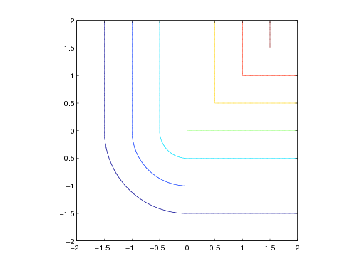
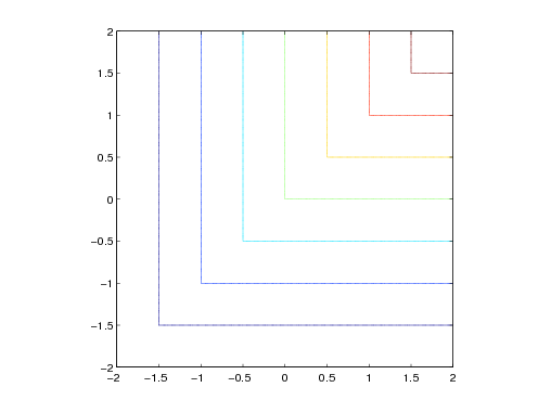
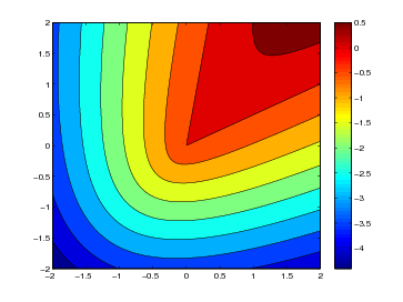
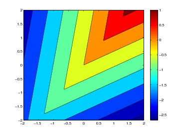
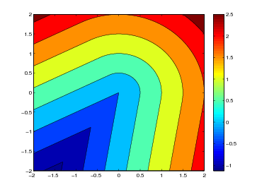
Figure 2 (left) illustrates some contour lines of the distance field to the boundary of the domain previously defined. The distance field is signed such that points inside the intersection of the halfspaces are positive and points outside are negative. Fig. 2 (right) shows some contour lines of the scalar field defined by min(x,y).
|
As illustrated by Fig. 2, the scalar field obtained by min corresponds to the Euclidean distance field everywhere except in the domain defined by: Q := {(x,y) : x < 0 & y < 0. For each point in that domain, the closest point on the boundary is the point obtained by the intersection of the two lines x = 0 and y = 0. Contour lines in that domain are circular arcs centered at this point.
The expression of Q for two orthogonal halfspaces is simple. We need now to define it for any general shapes to be intersected and then explain how to compute the closest point on the surface in that domain.
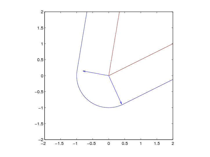
Figure 3 illustrates the case of the local intersection of two general (non orthogonal) curves intersecting at a point O. The boundary (d = 0), one contour line (d = -1.0) and the normals to each curve at O are drawn.
|
|
| Figure 3. Local intersection of two general curves. Boundary curve (red) resulting from the intersection, the contour line at the distance -1.0 (blue) and the normals to each curve at the intersection point. |
If the closest point is known, then the region of interest can be identified using the normal to each curve at the intersection point as seen in Fig. 3. However, since it requires to know the closest point, this method is not feasible. Instead, we proceed in the reverse way by first determining the domain of interest and then computing the closest point in that domain.
Given a point p R2 or R3 (see Fig. 4 for an illustration in two dimensions),
we first compute the projection p1 of p on the first curve c1. Using the signed
distance field d1 to the curve and its gradient ∇d1(p), the projection is given
by:
 |
(5) |
Similarly, we compute p2 the projection of p on the second curve c2. p belongs to the zone of interest Q, if d1(p2) < 0 and d2(p1) < 0.
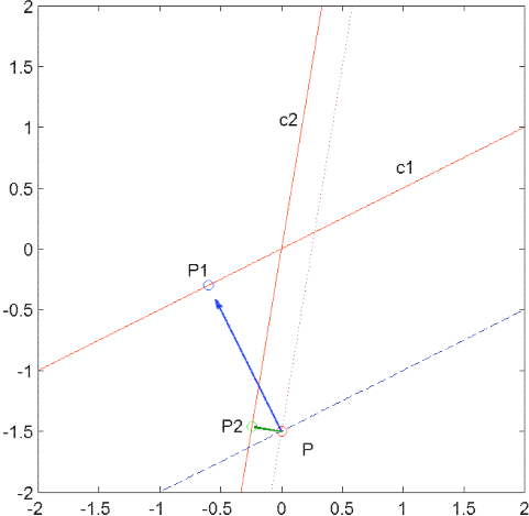
|
| Figure 4. Two curves c1 and c2 (solid lines) defined by the iso-lines of the distance fields d1 = 0 and d2 = 0. A given point p and the contour lines of d1 and d2 passing through p. p1 and p2 the projections of p on c1 and c2. |
After determining if a point is in the domain where min applied to the distance fields differs from the Euclidean distance field, we need to determine the closest point on the boundary of the solid obtained by the intersection of the two solids.
In all the above examples, the closest point on the boundary of the intersection from a point in the domain Q happened to be at the intersection of the two curves. This is not always the case. The closest point (x,y,z) on the boundary of the intersection of S1 and S2 from a point (x0,y0,z0) in Q is the solution to the following constrained optimization problem:
| Minimize: |  |
(6) |
| such that: | d1(x,y,z) ≥ 0 | (7) |
| and: | d2(x,y,z) ≥ 0 | (8) |
Where: d1 and d2 are the distance fields to the boundary of the solids S1 and S2. In Mathematicatm [22], such a constrained minimization problem can be solved with the command NMinimize. The point (x0,y0,z0) can be used as a starting point. Since this point is in general close to the solution, the convergence is relatively fast.
Regrouping all the results obtained so far, a procedure for computing the distance to the boundary of the intersection of two solids defined by signed distance functions is:
1: function INTERSECTION(p,d1,d2) 2: vd1 = d1(p) 3: vd2 = d2(p) 4: n1 = ∇d1(p) 5: p1 = p - vd1n1 6: n2 = ∇d2(p) 7: p2 = p - vd2n2 8: inQ = d1(p2) < 0 AND d2(p1) < 0 9: if inQ is true then 10: pc = solution of (6) subject to constraints (7) and (8) 11: vd = -∥p - pc∥2 12: else 13: vd = min(vd1,vd2) 14: end if 15: return vd 16: end function |
Modification of the previous algorithm for obtaining the distance to the difference of two solids consists in replacing the function d2(.) by the function -d2(.) everywhere.
For the union, the following changes need to be made to the previous algorithm for the intersection:
Finally, the closest point computed in line 9 is obtained by solving the following constrained minimization problem:
| Minimize: |  |
(9) |
| such that: | d1(x,y,z) ≤ 0 | (10) |
| and: | d2(x,y,z) ≤ 0 | (11) |
Scalar fields corresponding to the intersection and union of two solids is illustrated in two and three dimensions in the following examples. Min/max, R-functions and the methods described in this paper are used to compute these scalar fields.
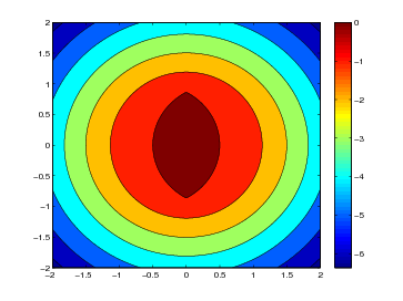
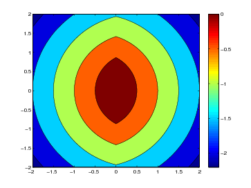
Figure 5 illustrates the contour plot of signed distance functions obtained by the intersection of two non-orthogonal planes and by the intersection of two disks. Intersection was implemented using: R-functions (left), min/max (middle) and the method proposed in this paper (right). The functions built using R-functions clearly differ from the Euclidean distance to the boundary of the constructed solid. The functions built using min/max fail also to do so but only in a subset of R2. In comparison, the method described in this paper allows the construction of an accurate signed distance field to the boundary of the constructed solids as illustrated by the circular arcs in the contour lines outside of the constructed solids.
|
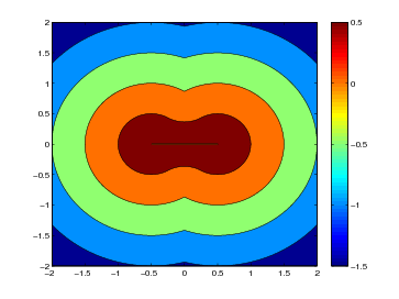
Figure 6 illustrates contour plots of the distance fields to the boundary of the union of two halfplanes (left) and two disks (right) using the method introduced here.
|
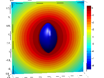
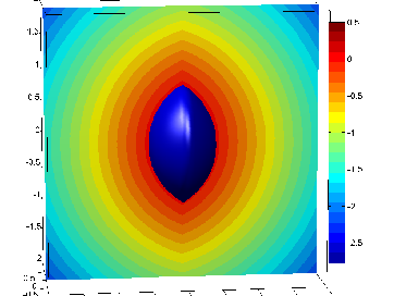
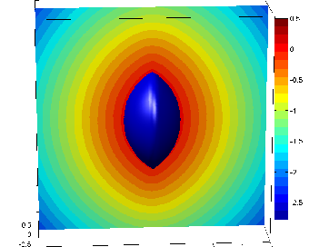
Visualizing scalar fields in three dimensions is more difficult. We visualize instead contour plots of the fields in a planar section. Fig. 7 (right) illustrates the proposed method applied in three dimensions to compute the distance to the intersection of two spheres. Contour plots need to be compared with the contour plots shown in fig. 7 (left) and (middle) obtained with respectively R-functions and min.
|
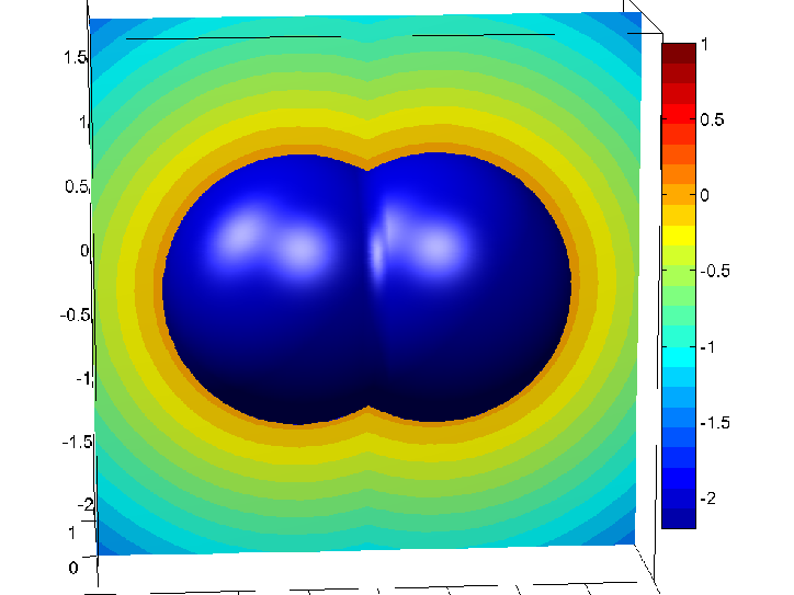
Figure 8 illustrates the result of the proposed method to compute the distance to the union of two spheres by showing a contour plot of the constructed distance field on a section by the plane y = 0.
The distance function is continuous but not everywhere differentiable; for example: the function d(p) = 1 -∥p - pc∥2 is not differentiable at the point p = pc. The algorithms described above use the gradient of the functions passed as arguments. Points at which the gradients can not be computed need to be handled differently. These points are on the medial axis of the solid and have more than one closest point on the surface of the solid. A possible solution is to select one of the closest point on the surface and define the gradient as the unit vector ending at this point.
It is possible to successively apply the proposed methods for intersection,
union or difference to solids built using these operations. The gradient of
the function constructed by the methods described in this paper needs
to be computed. In the example of the intersection, the function is not
differentiable at the points: {p : p Q and d1(p) = d2(p)}. This point-set
corresponds to the medial axis of the resulting solid. It is possible to use
the same method as described above. An alternative solution is to use
modified versions of min and max. In the case of min, it is possible to write: min(d1,d2) =
Q and d1(p) = d2(p)}. This point-set
corresponds to the medial axis of the resulting solid. It is possible to use
the same method as described above. An alternative solution is to use
modified versions of min and max. In the case of min, it is possible to write: min(d1,d2) =  (d1 + d2 +
  ) and to add a small perturbation ϵ:
  (d1,d2) =
  (d1 + d2 +
  ). This function is C1 however it has the
inconvenient of displacing each iso-contour; for example: assuming that d1 = 0 and d2 > 0, then
). This function is C1 however it has the
inconvenient of displacing each iso-contour; for example: assuming that d1 = 0 and d2 > 0, then  (d1,d2) =
  (d2 +
(d2 +  ) < 0 instead of 0.
The proposed expressions for the set operations are in general slower than min/max or the corresponding R-functions. This is due to the necessity to solve a constrained minimization problem in some cases. We have only done experiments with the NMinimize function of Mathematicatm and some simple algorithms to solve this minimization problem. Since the objective function is not too complicated, there should be some more efficient methods. In addition, it is possible to provide a good approximate guess for the starting point, making the convergence relatively fast.
We have presented in this paper algorithms for computing in two and three dimensions the distance to a solid obtained by applying set operations (intersection, union or difference) to primitives. Contrary to the existing implementations of these operations (min/max and R-functions), the proposed methods allow to compute the signed Euclidean distance field to the boundary of the resulting shape.
We are considering extending this work by experimenting with the iterative application of these operations in order to construct complex solids. The use of these functions should also allow to easily implement rolling ball blend and double offsetting.
[1] L. Barthe, N. A. Dodgson, M. A. Sabin, B. Wyvill, and V. Gaildrat. Two-dimensional potential fields for advanced implicit modeling operators. Computer Graphics Forum, 22(1):23–33, 2003.
[2] A. Biswas, V. Shapiro, and I. Tsukanov. Heterogeneous material modeling with distance fields. Comput. Aided Geom. Des., 21(3):215–242, 2004.
[3] J. Bloomenthal, editor. Introduction to Implicit Surfaces. Morgan-Kaufmann, 1997.
[4] P.-A. Fayolle, A. Pasko, B. Schmitt, and N. Mirenkov. Constructive heterogeneous object modeling using signed approximate real distance functions. Journal of Computing and Information Science in Engineering, 6(3):221–229, 2006.
[5] J. Hart. Sphere tracing: A geometric method for the antialiased ray tracing of implicit surfaces. The Visual Computer, 12(10):527–545, 1996.
[6] J. C. Hart. Distance to an ellipsoid. In P. Heckbert, editor, Graphics Gems IV, pages 113–119. Academic Press, Boston, 1994.
[7] K. Hoff, T. Culver, J. Keyser, M. Lin, and D. Manocha. Fast computation of generalized voronoi diagrams using graphics hardware. In Proceedings of ACM SIGGRAPH, pages 277–286. ACM, 1999.
[8] P.-C. Hsu and C. Lee. The scale method for blending operations in functionally-based constructive geometry. Computer Graphics Forum, 22(2):143–158, 2003.
[9] M. Jones and M. Chen. A new approach to the construction of surfaces from contour data. Computer Graphics Forum, 13(3):75–84, 1994.
[10] S. Mauch. Efficient Algorithms for Solving Static Hamilton-Jacobi Equations. PhD thesis, California Institute of Technology, 2003.
[11] A. Pasko, V. Adzhiev, A. Sourin, and V. Savchenko. Function representation in geometric modeling: concepts, implementation and applications. The Visual Computer, 8(11):429–446, 1995.
[12] A. Pasko and V. Savchenko. Blending operations for the functionally based constructive geometry. In set-theoretic Solid Modeling: Techniques and Applications, CSG 94 Conference Proceedings, pages 151–161. Information Geometers, 1994.
[13] B. Payne and A. Toga. Distance field manipulation of surface models. IEEE Computer Graphics and Applications, 12(1):65–71, 1992.
[14] A. Ricci. A constructive geometry for computer graphics. The Computer Journal, 16(2):157–160, 1973.
[15] C. Roessl, F. Zeilfelder, G. Nurnberger, and H.-P. Seidel. Spline approximation of general volumetric data. In Proceedings of ACM Solid Modeling. ACM Solid Modeling 2004, 2004.
[16] J. Rossignac and A. Requicha. Constant-radius blending in solid modeling. Computers in Mechanical Engineering, 3(1):65–73, 1984.
[17] V. Rvachev. Theory of R-functions and Some Applications. Naukova Dumka, Kiev, 1982. In Russian.
[18] M. Sabin. The use of potential surfaces for numerical geometry. Technical Report VTO/MS/153, British Aircraft Corporation, 1968.
[19] J. Sethian. Level-Set Methods and Fast Marching Methods. Cambridge University Press, 1999.
[20] A. Sud, A. Otaduy, and D. Manocha. Difi: Fast 3d distance field computation using graphics hardware. Computer Graphics Forum, 23(3):557–566, 2004. Proceedings of Eurographics 2004.
[21] Y. Tsai. Rapid and accurate computation of the distance function using grids. J. Comput. Phys., 178(1):175–195, 2002.
[22] Wolfram Research Inc. Mathematica Edition: Version 7.0. Wolfram Research, Inc., 2008.
[23] H. Zhao. A fast sweeping method for eikonal equations. Mathematics of Computation, 2004.
[24] Y. Zhou, A. Kaufman, and A. Toga. 3d skeleton and centerline generation based on an approximate minimum distance field. The Visual Computer, 14(7):303–314, 1998.
П. Файоль
А. Пасько*
Университет Айзу, Япония
* Университет Борнмута, Великобритания
Представлены методы вычисления Евклидового расстояния со знаком и визуализации поверхностей тел, полученных с помощью пересечения, объединения и вычитания твердых тел. Такой подход позволит заменить функции min/max и R- функции, традиционно используемые для описания теоретико-множественных операций.
Ключевые слова: моделирование форм и твердых тел, конструктивное моделирование