general implementation Aspects of the Gpu-based volume rendering algorithm
N. GAVRILOV, V. TURLAPOV
gavrilov86@gmail.com, vadim.turlapov@cs.vmk.unn.ru
Lobachevsky state university of Nizhny Novgorod, Russia
Contents:
1. Introduction
1.1 The framework development motivation
1.2 Visualization software survey
2.1.1 Maximum Intensity Projection (MIP)
2.1.2 The shaded Direct Volume Rendering (DVR)
2.1.3 Semi-transparent iso-surfaces
2.2.1 Early ray termination
2.2.2 Empty space skipping via the acceleration structure
2.2.3 Empty space skipping via the volumetric clipping
2.3 Rendering artifacts reduction
2.4 Data processing algorithms
3. Visualization performance results
4. Conclusions
This paper presents GPU-based algorithms and methods of the Direct Volume Rendering (DVR) we have implemented in the “InVols” visualization framework (http://ngavrilov.ru/invols). InVols provides new opportunities for scientific and medical visualization which are not available in due measure in analogues: 1) multi-volume rendering in a single space of up to 3 volumetric datasets determined in different coordinate systems and having sizes as big as up to 512x512x512 16-bit values; 2) performing the above process in real time on a middle class GPU, e. g. nVidia GeForce GTS 250 512 MB; 3) a custom bounding mesh for more accurate selection of the desired region in addition to the clipping bounding box; 4) simultaneous usage of a number of visualization techniques including the shaded Direct Volume Rendering via the 1D- or 2D- transfer functions, multiple semi-transparent discrete iso-surfaces visualization, MIP, and MIDA. The paper discusses how the new properties affect the implementation of the DVR. In the DVR implementation we use such optimization strategies as the early ray termination and the empty space skipping. The clipping ability is also used as the empty space skipping approach to the rendering performance improvement. We use the random ray start position generation and the further frame accumulation in order to reduce the rendering artifacts. The rendering quality can be also improved by the on-the-fly tri-cubic filtering during the rendering process. InVols supports 4 different stereoscopic visualization modes. Finally we outline the visualization performance in terms of the frame rates for different visualization techniques on different graphic cards.
KEYWORDS
GPGPU, ray casting, direct volume rendering, medical imaging, empty space skipping.
In scientific visualization it is often necessary to deal with some volumetric regular scalar datasets. These data may be obtained by some numerical simulation or via the scanning equipment such as tomographs. The output data of the CT scan is a series of the slices, i.e. two-dimensional scalar arrays of 16-bit integer values. The stack of such slices can be interpreted as a volumetric dataset which can be visualized as some 3D object.
Since the 90s, the Direct Volume Rendering shows itself as an efficient tool for the visual analysis of volumetric datasets [4]. Different established approaches [1] make possible the implementation of the real-time volume rendering by using the parallel and high-performance computations on the GPU. The recent progress in GPGPU computations makes the real-time multi-volume rendering possible [2]. In this paper we make a review of some general details of DVR and other algorithms we have implemented in our InVols viewer for the multi-volumetric datasets visual exploration.
1.1 The framework development motivation
During our collaboration with the Institute of Applied Physics of the Russian Academy of Sciences (http://www.iapras.ru/) there was a need to make a volumetric visualization of the molecular dynamic simulation of the electron bubble transport process (Figure 1.a, f, g). There was a number of different volumetric datasets being obtained during this simulation, representing different scalar and vector fields. These datasets could be visualized together, in one space. Actually, there was a need to visualize two scalar fields – the electrons’ density and the electrical field absolute value. However, there was no scientific visualization software available, which could satisfy our needs in the visual analysis of the scientific multi-volume and time-varying volumetric datasets we had. On the other hand, the high quality and performance visualization of the large multi-modal volumetric medical datasets is also needed in ours university telemedicine project (http://www.unn.ru/science/noc.html).
We also wanted to be able to add several desired specific features in our own visualization framework. For instance, the interactive volumetric section via the arbitrary polygonal mesh can be efficiently used for the interactive and suitable selection of the region of interest, and we have not found any solutions with this feature.
There is no multi-volume rendering software available as well, so its development is still in the research domain. The multi-volume rendering for the medical imaging is a rendering in a single space of several volumetric datasets determined in different coordinate systems and usually having sizes as big as up to 512x512x512 16-bit values. Performing the above process in real time on a middle class GPU (e. g. nVidia GeForce GTS 250 512 MB) is provided by the acceleration techniques we propose in this paper.
One of the considerable problems in the scientific visualization is a settings tuning complexity. In order to give the user an ability to choose between the predefined visualization settings by comparing the corresponding resulting images we decided to implement the simultaneous rendering by a number of visualization techniques including the shaded Direct Volume Rendering via the 1D- or 2D- transfer functions, multiple semi-transparent discrete iso-surfaces visualization, MIP, and MIDA.
Below we make a review of some significant visualization software solutions we have encountered.
1.2 Visualization software survey
There are many free or even open-source software products for medical and scientific volumetric visualization. The Voreen (Volume Rendering Engine) is an open source volume rendering engine, which allows interactive visualization of volumetric data sets with high flexibility when integrating new visualization techniques. It is implemented as a multi-platform (Windows, Linux, Mac) C++ library using OpenGL and GLSL for GPU-based rendering, licensed under the terms of the GNU General Public License. To see what Voreen can do, take a look at the video tutorials, the gallery, the getting started guide, or just download Voreen and try it out yourself (http://www.voreen.org/).
The Voreen demo can be nicely used for some scientific datasets visualization and the rendering quality is good enough. But when dealing with some big dataset (e.g. 512x512x512 cells) it appears to be hardly a real-time visualization. Moreover, there is no support for the multi-volume datasets rendering, when we want to render several datasets together in one space. There are also other motivations to implement our own volumetric viewer rather than remodel the Voreen core: rendering quality improvement, different stereoscopic rendering modes, embedded interactive segmentation, etc.
The other significant visualization software is the OsiriX viewer (http://osirix-viewer.com), an image processing software dedicated to DICOM images (".dcm" / ".DCM" extension) produced by imaging equipment (MRI, CT, PET, PET-CT, SPECT-CT, Ultrasounds, ...). OsiriX has been specifically designed for navigation and visualization of multimodality and multidimensional images: 2D Viewer, 3D Viewer, 4D Viewer (3D series with temporal dimension, for example: Cardiac-CT) and 5D Viewer (3D series with temporal and functional dimensions, for example: Cardiac-PET-CT). The 3D Viewer offers all modern rendering modes: Multiplanar reconstruction (MPR), Surface Rendering, Volume Rendering and Maximum Intensity Projection (MIP). All these modes support 4D data and are able to produce image fusion between two different series.
The OsiriX viewer is designed for the medical staff and has a lot of features, but it is the MacOs-only software. And while it is the medical imaging software, it can be hardly used for the scientific data visualization, because the user may want to obtain some specific data visual representation. The medical data format has its own specific, which is considered when implementing the medical imaging algorithms:
1) For the CT dataset there are only 12 first bits used;
2) The data cells with minimal values are usually located outside rather than inside the volumetric dataset;
3) The dataset areas with maximal data values are usually needed to be visualized (bones, soft tissues), while the minimum is often to be transparent (air, non-scanned areas in the slices’ corners).
Fovia Inc. (http://fovia.com), headquartered in Palo Alto, California, has developed High Definition Volume Rendering®, a proprietary, software-only volume rendering technique that delivers unparalleled quality and performance. Volume rendering has become invaluable for a wide variety of applications in many fields, including medical, dental, veterinary, industrial, pharmaceutical and geoscience. Fovia’s HDVR® software is more scalable, cost effective, flexible, and easily deployable on an enterprise-wide basis than are GPU or other hardware-based approaches.
The Fovia’s CPU-based Ray Casting efficiency shows that even such GPU-suitable algorithms, like the Ray Casting, are still may be implemented fully on the CPU with the same or better results. However, while the graphical cards’ performance, availability and architecture flexibility increases, the CPU-based efficient Ray Casting implementation is a very difficult task. It is a question of time when the huge datasets may be fully loaded into the GPUs memory. Besides, the Fovia is hardly acceptable for the free usage and has no desired features like multi-volume rendering and polygonal mesh based volumetric clipping.
2. METHODS AND ALGORITHMS
In this section we make a brief inspection of the Ray Casting and some other algorithms we have implemented in our system. All of these algorithms efficiently use a GPU and are implemented via the shader programs. All the GLSL-shader programs of the InVols framework are available as the text files with extension FS and may be downloaded with the InVols demo from our internet resource http://ngavrilov.ru/invols. You can also find the screenshot gallery, documentation and some video there.
Due to the high flexibility of the Ray Casting (RC) method there is a huge amount of different possible visualization techniques. The RC algorithm calculates each pixel of the image by generating (casting) rays on the screen plane and traversing them towards the observer viewing direction. Each of the RC-based rendering algorithms takes the ray start position and its direction as the input parameters, and the pixel color as the algorithm output.
There are six rendering techniques in the InVols framework and each of them supports multi-volume rendering, i.e. these algorithms can handle up to 3 volumetric datasets, which are arbitrary located in the world space. The dataset’s location is determined by the transformation 3x4 matrix. In addition to the volume’s position and orientation, this matrix also defines the spacing by x, y and z components, which allows for the proper volume scaling. So to perform a sampling from the arbitrary located dataset we multiply the sampling point by this matrix, so we’ll get the sampling point in the volume’s local coordinate system.
In order to perform the GPU-based Ray Casting, we use GLSL shaders to calculate the screen plane’s pixels’ colors, like it is done in the Voreen framework. Each of the rendering methods in our framework is defined by some GLSL fragment shader program, i.e. a text file with the GLSL code. These methods differ from each other, but they uniformly handle all visualization parameters of the InVols, e.g. the observer position, transfer functions, iso-surfaces, anaglyph matrix, etc. So it is easy for us to add new RC-based rendering techniques in the InVols. The framework allows for the simultaneous rendering by a number of visualization techniques including the shaded Direct Volume Rendering via the 1D- or 2D- transfer functions, multiple semi-transparent discrete iso-surfaces visualization, MIP, MIDA, etc.
2.1.1 Maximum Intensity Projection (MIP)
The Maximum Intensity Projection (MIP) is one of the most popular volumetric visualization techniques in the medical imaging [5]. It is easy for clinicians to interpret an MIP image of blood vessels. By analogy the Minimum Intensity Projection (MinIP) may be used for bronchial tube exploration.
As one can guess by the caption, the maximal intensities of the volumetric dataset are projected onto the screen plane. Usually the projected intensity determines the pixel’s color in the gray-scaled manner (Figure 1c). It medical imaging there is a window/level concept. The window is represented by two scalar values – the window width and window center.
2.1.2 The shaded Direct Volume Rendering (DVR)
The shaded DVR technique is also used in a medical exam, but its usage is more limited [4]. In contrast to the MIP technique here we can use the early ray termination approach, which considerably improves the rendering performance without any image visible changes. This termination can be done because of the DVR algorithm nature – while traversing throw the volume data, the ray accumulates color and opacity, i.e. the optical properties, defined by the transfer function (TF). While the opacity increases, the contribution to the final pixel’s color decreases. This opacity accumulation is commonly used to visualize the data as a realistic volumetric object.
By default it is implied that the one-dimensional transfer function is used to map the data values onto the colors and opacities. It is also implied that there is no shading, i.e. no local illumination model is used. The shading improves volumetric perception of an object. Using the multi-dimensional transfer functions may be useful when investigating some specific features in scientific volumetric data [6]. However both of these options require additional computational resources. For several 1D transfer functions we use a common 2D texture. There are 65536 possible data values (for the 16-bit data) while we use a texture width of 512 texels only. So we have to map our texture to some small data values’ range. To alter the transfer function a user adds the colored control points in the bottom window (Figure 1h).
For the two-dimensional transfer functions we use another approach: the parameterized transfer function, instead of the color table (here we would use two-dimensional textures). To assign the visual properties we use rectangular widgets in the arguments space. Usually the 2D-transfer function’s arguments are the data value itself and the gradient magnitude in the corresponding point.
2.1.3 Semi-transparent iso-surfaces
Semi-transparent iso-surfaces are usually used for the scientific data visualization, because these surfaces are easier to interpret when examining some new phenomena. One of the main advantages of this method over the DVR’s one is a surface’s visualization high quality: here we can search for more exact intersection with the surface, a so called Hitpoint Refinement [8], while in DVR there are no surfaces. There are opaque regions in DVR, but theirs accurate visualization requires more difficult algorithm, and its laboriousness considerably reduces the performance of the GPU-implementation.
This method searches for ray’s intersections with the iso-surfaces. When the ray passes across the iso-value, we calculate a more exact intersection point determined by the ray positions and sampled values on the current and previous steps. The linear interpolation is enough to obtain a desired result.
Each of the iso-surfaces is defined by several parameters: iso-value, color and opacity. These parameters are adjusted by the Transfer function window.
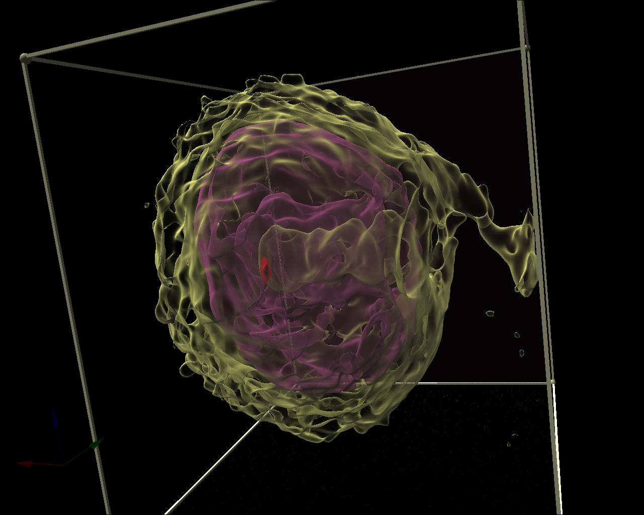
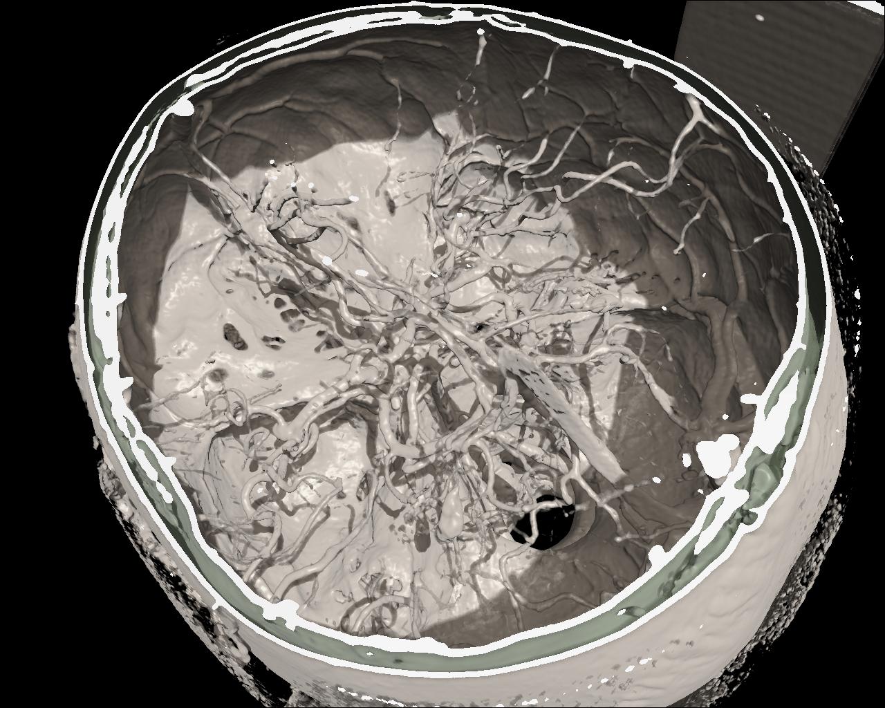
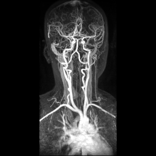
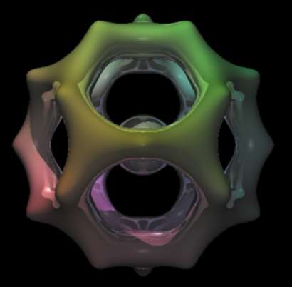
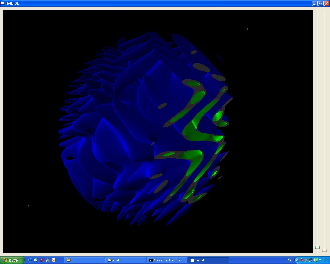
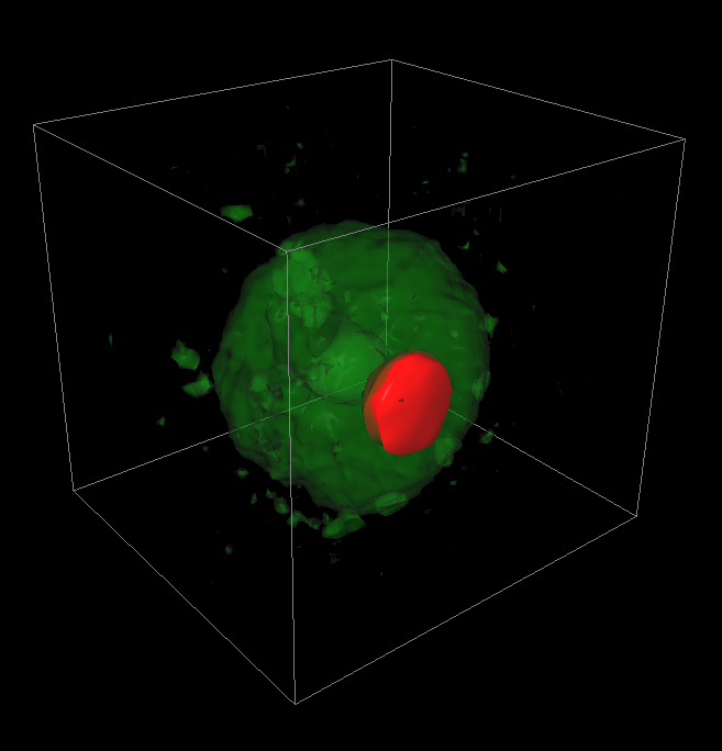
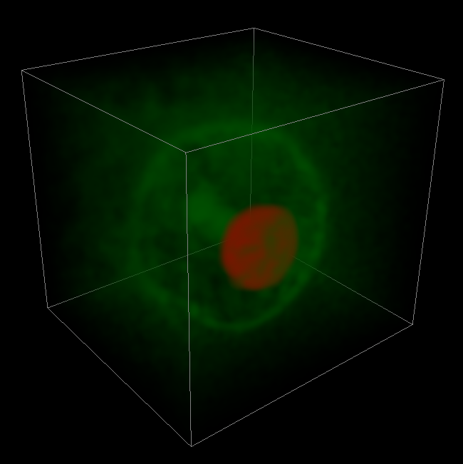
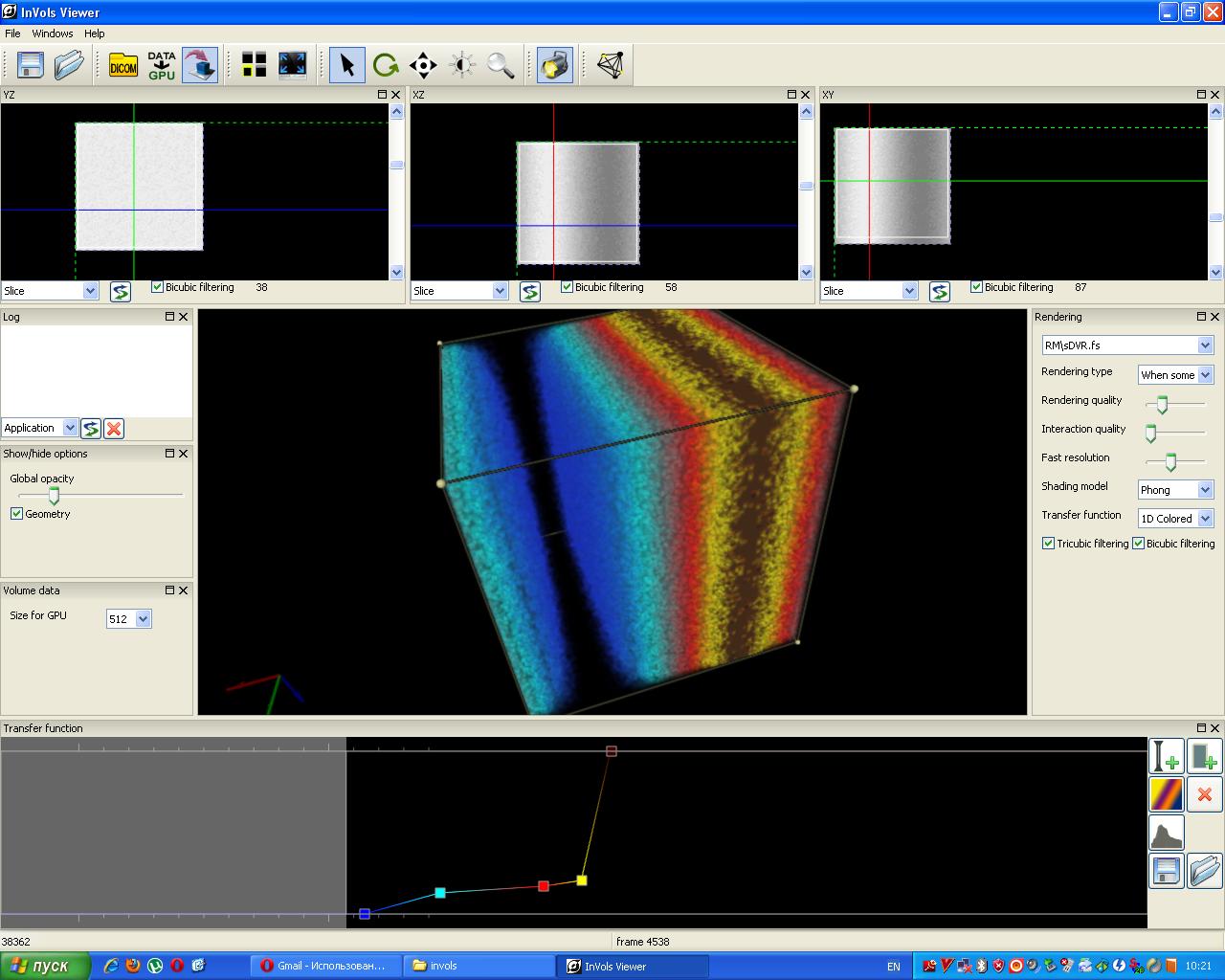
Figure 1. RC techniques: a) semi-transparent iso-surfaces for the scientific data; b) opaque iso-surface with shadows computation; c) MIP (the Maximum Intensity Projection); d, e) iso-surfaces for the scalar fields (defined by the formulas); f, g) iso-surfaces and DVR (Direct volume rendering) techniques for the same scientific dataset. The electrons’ density (green) and the electrical field absolute value (red); h) The InVols’ GUI.
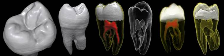
Figure 2. Different rendering of the same tooth dataset: a, b) DVR; c) 3 surfaces; d) 1 surface d) DVR via the 2D transfer function; e) 2 surfaces.
2.2 Optimization strategies
2.2.1 Early ray termination
The Early ray termination technique is a common optimization strategy for a Ray Casting algorithm. It is possible to terminate the RC algorithm for each individual ray if the accumulated opaqueness is close to 1. However, in rendering techniques like the MIP it is necessary to browse the whole ray path until leaving the bounding volume.
2.2.2 Empty space skipping via the acceleration structure
The Empty space skipping approaches are used extensively in CPU-based DVR [7]. However, some techniques can be extended to the GPU-implementation. We use two levels of volumetric data hierarchy: the source dataset, e.g. of size 512x512x512, and the acceleration structure, i.e. a small two-channel volumetric dataset of size 16x16x16. So each 32x32x32 block in the source data corresponds to one cell from the acceleration structure. Each of these cells contains minimum and maximum from the corresponding block in the source data. So for each block it is known, whether the corresponding space is transparent and may be skipped by a ray. This approach accelerates the visualization up to 1.5-2 times.
2.2.3 Empty space skipping via the volumetric clipping
The custom bounding polygonal mesh can be used either for the rendering acceleration [8] or for the data clipping, as an alternative to the dataset’s segmentation. We use OpenGL frame buffers to store the distances from the viewpoint to the mesh front and back faces. The buffers may contain up to 4 ray path segments (in [8] there is only one segment), so that the mesh is not required to be convex (Figure 3). Of course, before using these buffers we should fill them with some relevant data. To do it we draw the bounding mesh by calling common OpenGL instructions and perform rendering into the texture. We use a specific GLSL shader program to fill pixels with the relevant data instead of the standard OpenGL coloring. The program calculates the current distance between the observer and the fragment position. The only varying parameter is the fragment position, i.e. the point on the mesh surface. After the buffers are filled with the relevant distances, the Ray Casting may be performed (Figure 6). For each ray it is known, what segments of the ray path should be traversed.
Figure 3. The illustration of the volumetric clipping algorithm. The yellow regions of the screen plane identify pixels, where are only one path segment inside the bounding mesh. In the white region there are two path segments for the rays in the Ray Casting algorithm.
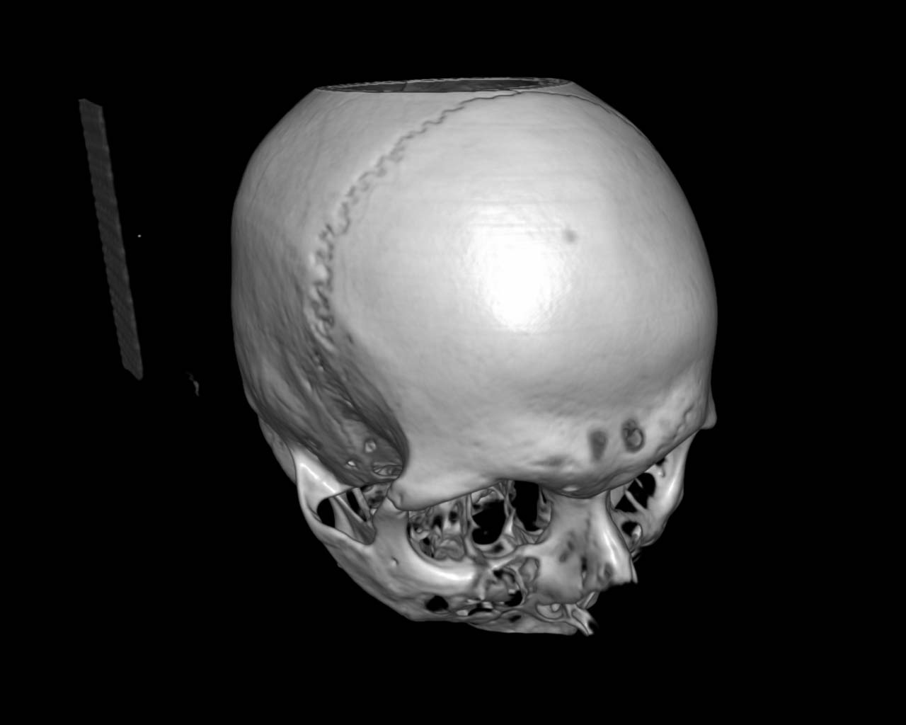
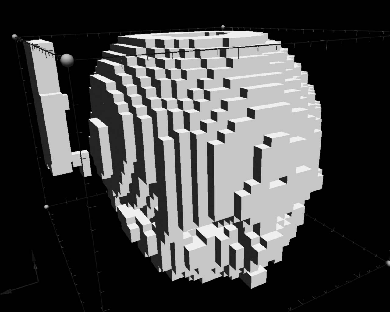
Figure 4. The source dataset (left) and its acceleration structure (right) visualization. Visible ‘bricks’ identify regions of interest that contain some visible features.
Figure 5. Empty space skipping: a) via the regular acceleration structure; b) via the bounding mesh
Figure 6. Back (red) and front (green) mesh faces. Rays should be moving only inside this mesh, i.e. from front to back mesh faces
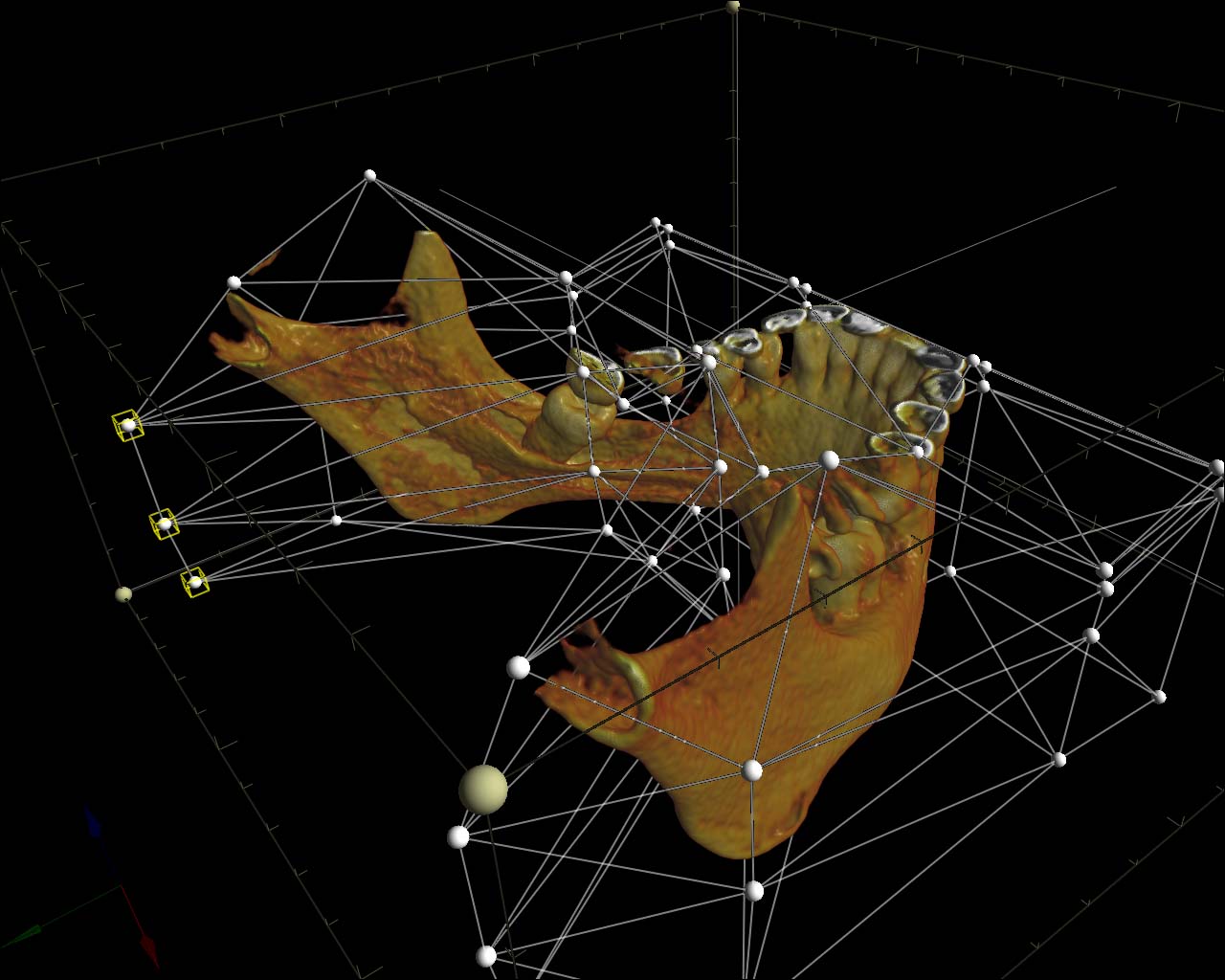
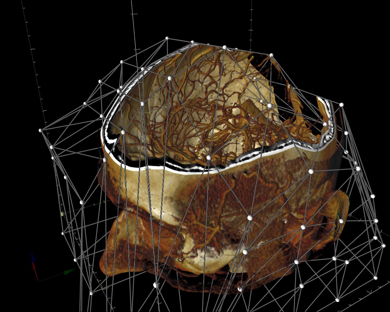
Figure 7. Volumetric data clipping via the custom polygonal mesh.
2.3 Rendering artifacts reduction
Because of the finite steps’ number the ray may skip some meaningful features in the dataset, even if the ray step is much less than the voxel’s size. As a result the ‘wood-like’ image artifacts may appear. This wood-likeness appears because each ray starts from the same plane (e.g. from the bounding box face). This artifacts’ regularity can be removed by randomization of the ray start positions (Figure 8). The final image will contain ‘noisy’ artifacts instead of ‘regular’ ones. If a user does not change the viewpoint and other visualization settings, these random frames can be accumulated by such a way that a user will see an average image that contains no noise (Figure 10).
Figure 8. Initial rays’ start positions randomization.
Figure 9. The random frames accumulation approach. Each ray has its own pattern of data samplings.
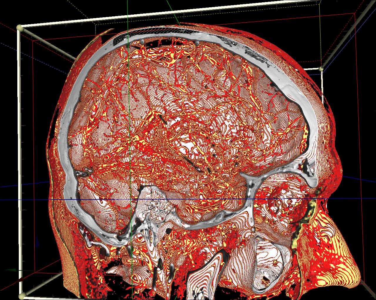
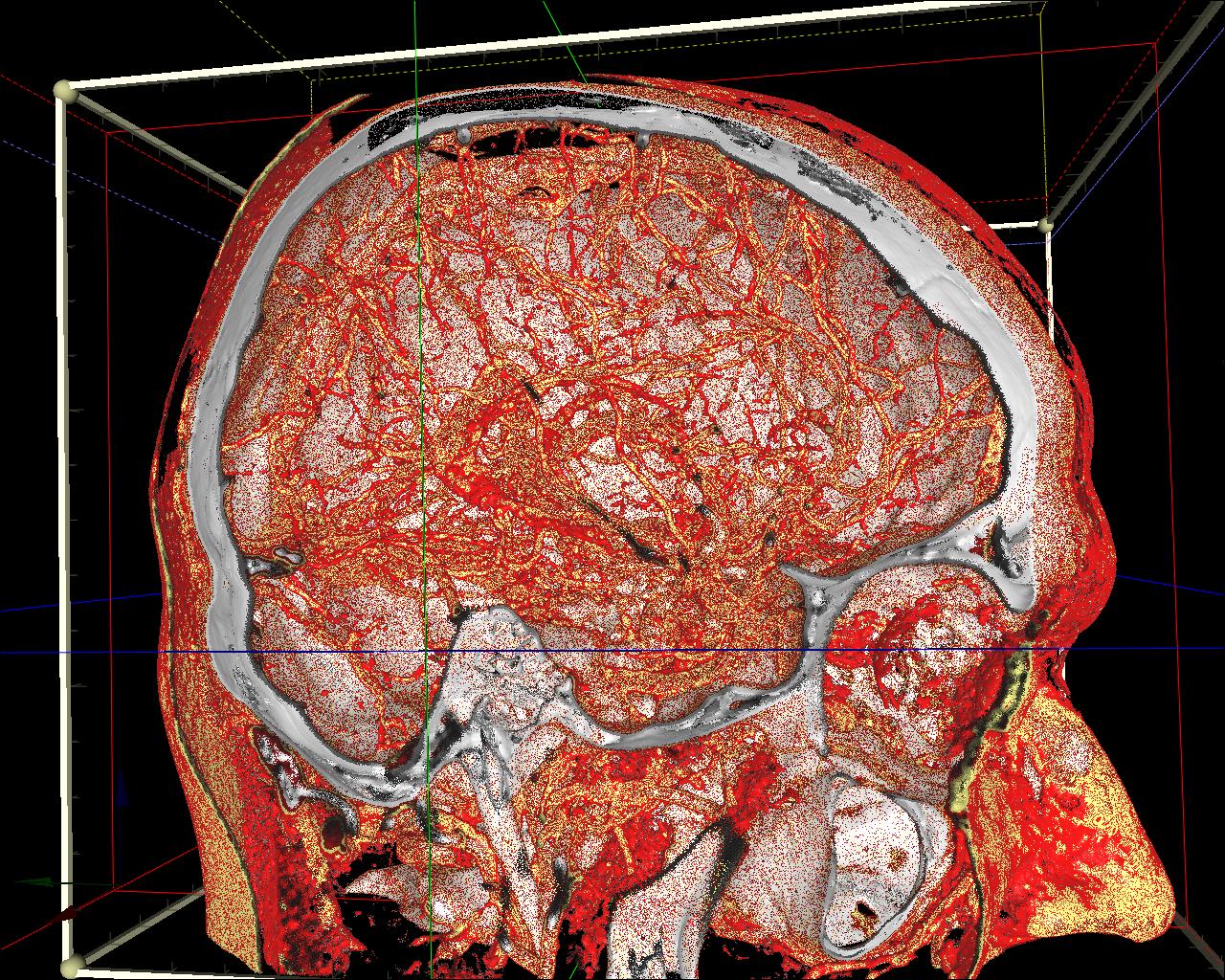
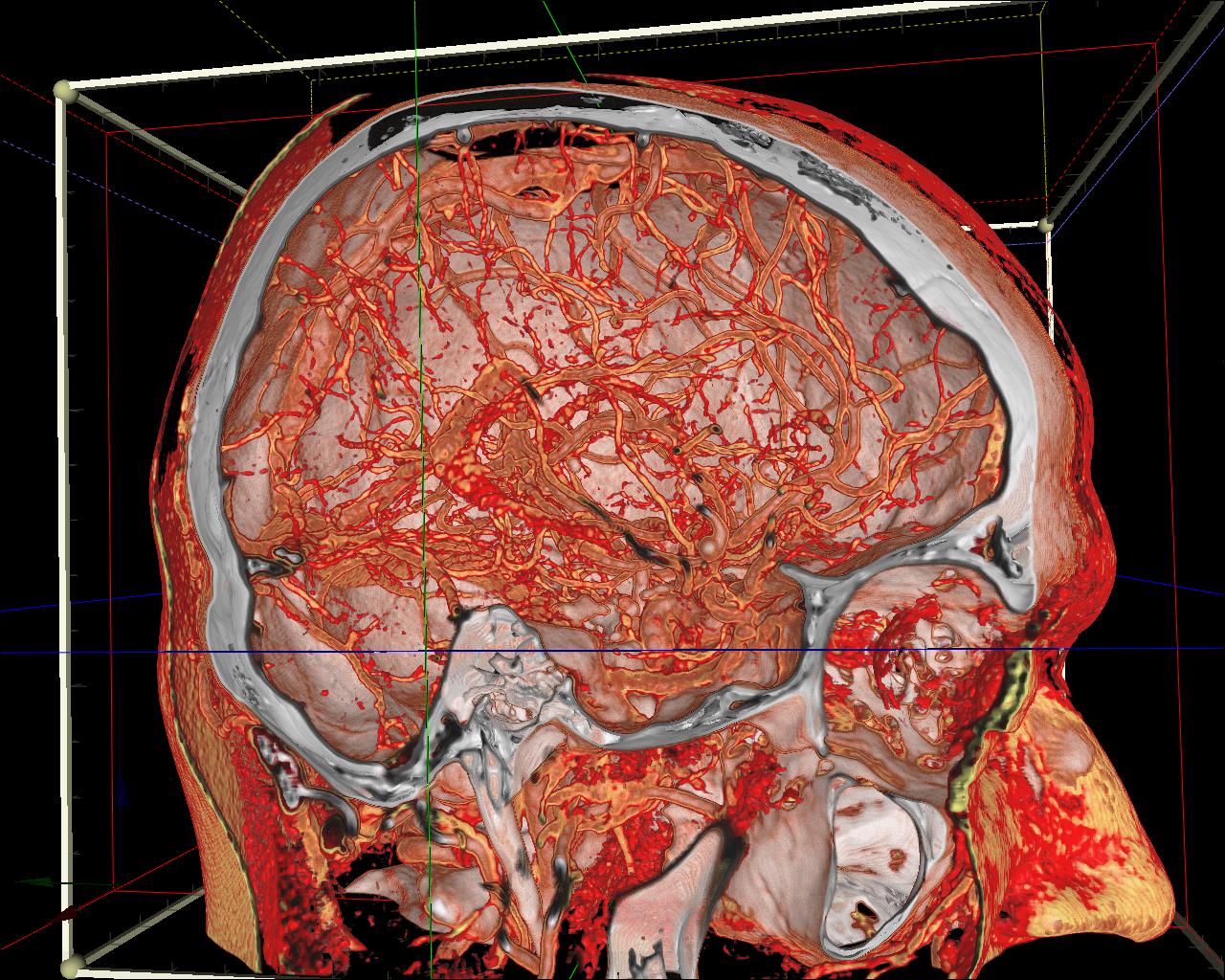
Figure 10. DVR ‘wood-like’ artifacts’ reduction: a) no reduction; b) artifact’s randomization; c) frames accumulation.
The visualization quality can be improved also via the tri-cubic filtering instead of the common tri-linear one. We have extended the algorithm for the two-dimensional case, presented in [3]. Considering the embedded bi-linear texture filtering ability, we can make only four samplings to calculate the bi-cubic interpolated value. In order to perform a single tri-cubic sampling it is necessary to make 8 basic tri-linear samplings from the same dataset, but in fact we will calculate the data value, determined by 64 nearest voxels’ values.
However, it is still rather costly to use this on-the-fly filtering in RC algorithm. However, if the dataset size is not very big (e.g. 256³ voxels or less) or if a rendering technique is simple enough (e.g. Direct Volume Rendering, opaque iso-surface) then the visualization will be interactive, i.e. over 20-30 fps.
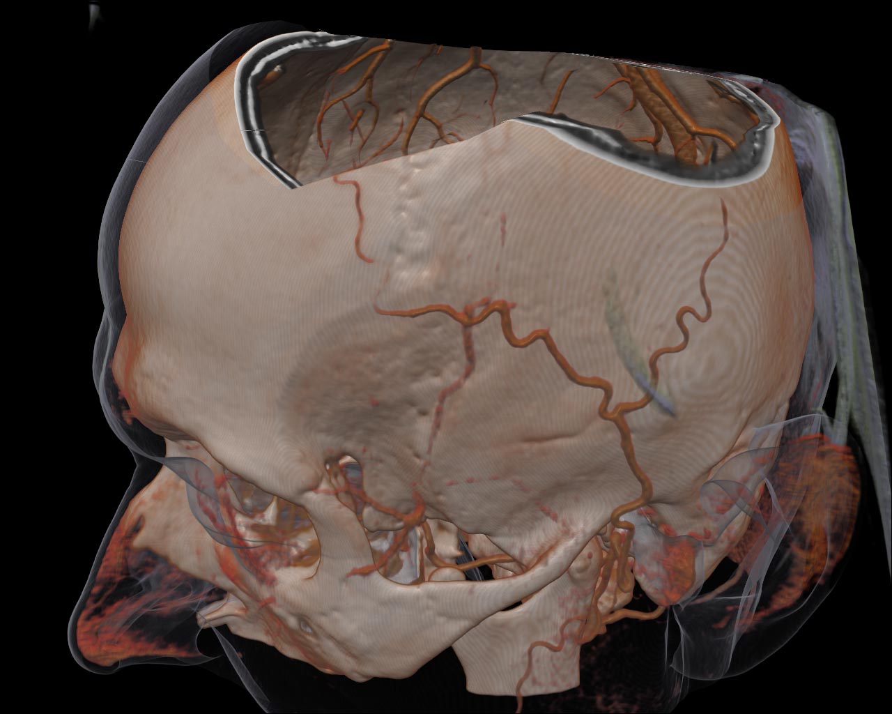
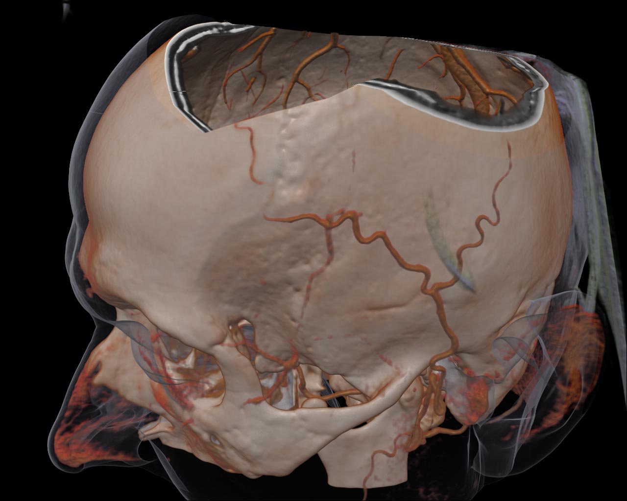
Figure 11. Different DVR on-the-fly sampling options, left: tri-linear filtering; right: tri-cubic filtering. Notice wood-like artifacts on the left figure.
2.4 Data processing algorithms
In order to improve visualization quality we have implemented a data resampling tool. A user can select any area from the data via the bounding box and resample this selection into another resolution. By default the resulting data is a resampled copy from the selected area in the source data. This processing is also implemented via the GLSL shaders, so the fragment shader defines the volumetric data processing algorithm. In the InVols there are additional operations with the data, like the Gaussian smoothing or median filter. There are also algorithms for generating other fields derived from the source data (e.g., the gradient magnitude field).
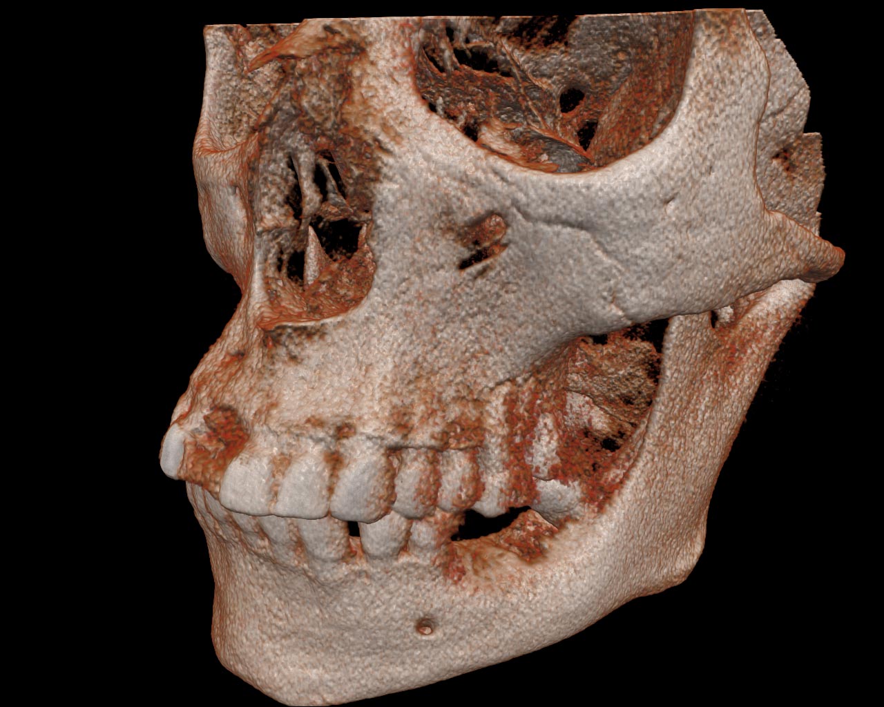
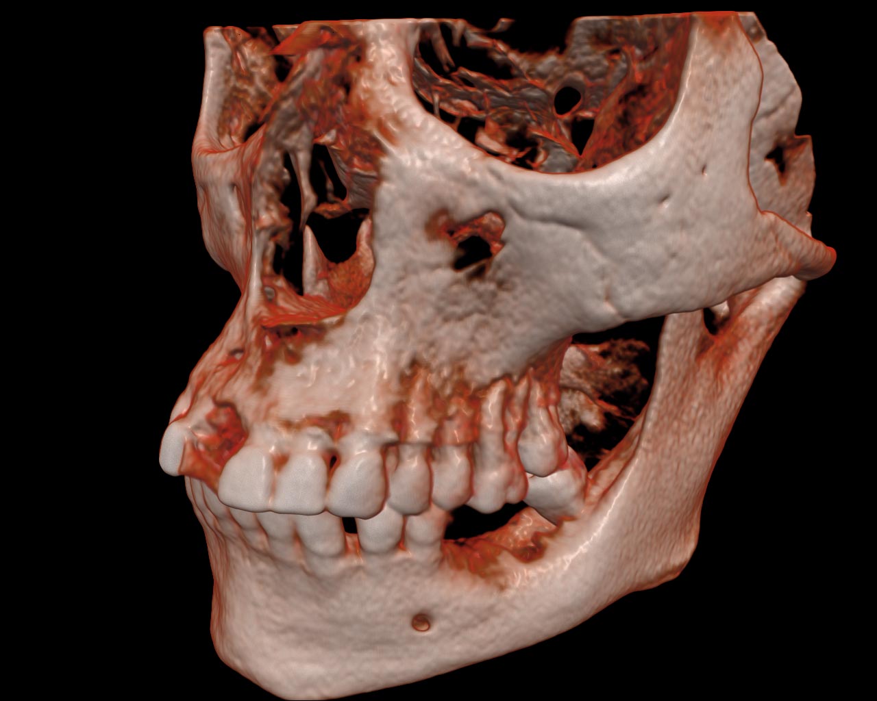
Figure 12. The DRV of the source CT-data (left) and the preprocessed one (right).
3. VISUALIZATION PERFORMANCE RESULTS
In table 1 we have outlined obtained volume rendering performance of the InVols for several graphic cards. We used a full screen resolution (1280x1024), 16-bit dataset of size 512x512x512, the ray step 0.0004 (i.e. 0.2 of the voxel size), and the viewpoint used in Figure 13a.
Table 1. Visualization performance for different rendering techniques in terms of frame rates (fps).
Isos means visualization of three semitransparent iso-surfaces
GPU |
DVR + Isos |
Isos |
MIP |
DVR |
Opaque iso-surface |
NVIDIA GeForce GTS 250 |
9 |
10 |
10 |
12 |
30 |
NVIDIA GeForce 9500 GT |
4 |
4 |
4 |
5 |
13 |
NVIDIA Quadro FX 5600 |
14 |
16 |
19 |
23 |
63 |
ATI RADEON HD 4870 |
18 |
21 |
35 |
38 |
81 |
ATI RADEON HD 4890 |
21 |
25 |
39 |
44 |
108 |
In general ATI cards overcome NVIDIA cards for the ray casting task. This can be explained by the fact, that the ATI cards have vector architecture, while ray casting algorithms contain many vector operations.
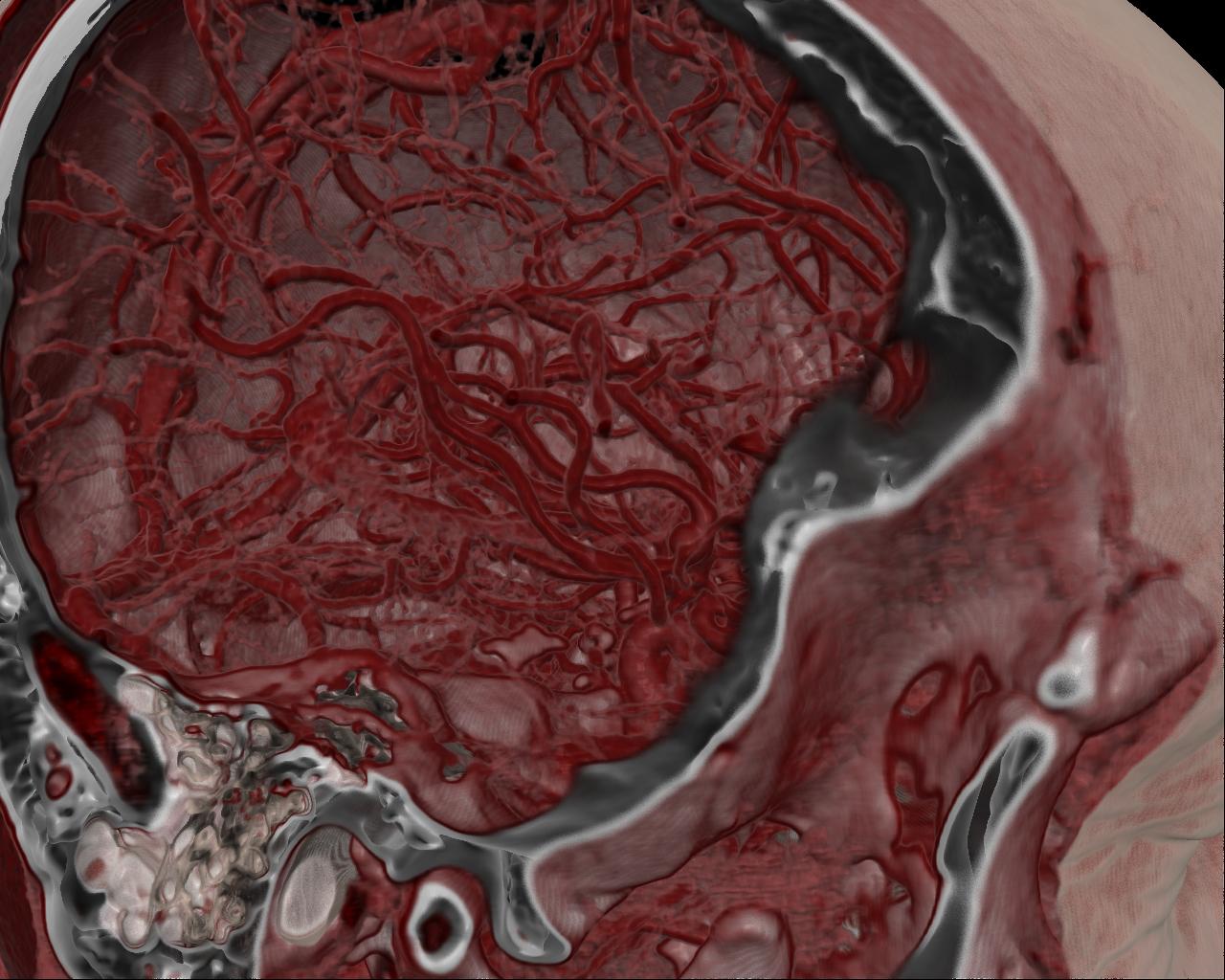
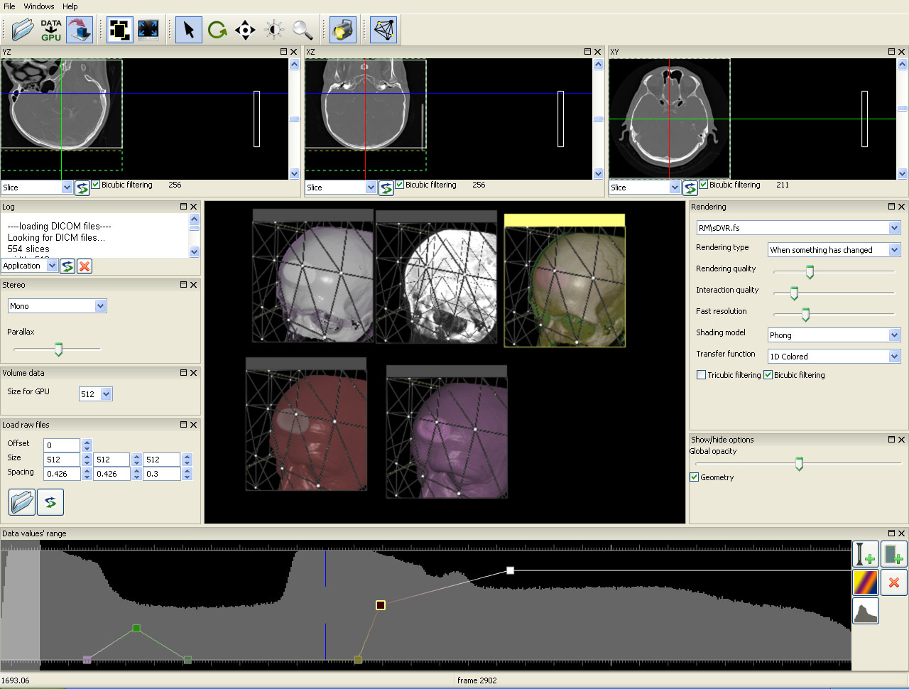

Figure 13. left to right: a) Brain blood vessels. Test viewpoint. b) InVols’ GUI. c) Multi-volume rendering of 3 datasets of sizes 512³ each.
4. CONCLUSIONS
The proposed framework can be used for the multi-modal medical data examination. A user can load datasets of the CT and MRI modalities as DICOM slices. Each dataset is determined be own coordinate system and a user can properly place them together in the space via the control points, so that the user sees the comprehensive 3D-picture of the medical examination. The real-time rendering is performed on middle level graphic cards (nVidia GeForce GTS 250 512 MB).
The framework supports four different stereoscopic visualization modes, so it may be used for stereo demonstrations via the stereo-pare of projectors, anaglyph, interlaced rendering or stereo-monitors (like Zalman with passive polarized glasses) or with shutter glasses via the nVidia 3D Vision technology.
The other meaningful InVols advantage over other similar software solutions is the volumetric clipping option. This clipping is performed via the arbitrary polygonal mesh. The triangles number is not sufficient and do not impair the rendering performance, so the mesh may have a rather complex structure and may be fitted to the visible features in the space. The clipping may be used either for the performance improvement or for the interactive manual data segmentation in order to select the volumetric region of interest. We define the bounding mesh as the triangulated visible cells of the regular acceleration structure (Figure 4). Here is the video devoted to this meshing: http://www.youtube.com/watch?v=3tPPzWmY2DM. This acceleration technique improves the rendering performance up to 2 – 4 times.
There are some other features which distinguish our framework from the others: the frames accumulation technique, the on-the-fly tri-cubic filtering option, the Ray Casting algorithm flexibility, which allows for the various visualization techniques implementation. Here is the one of the video demonstrating available rendering modes: http://www.youtube.com/watch?v=DtqiiJitgBU.
In the near future we are going to implement the huge datasets visualization (over 512³). In our opinion, it is one of the most considerable problems in the GPU-based DVR. Today the CPU-based DVR via the Ray Casting overcomes the GPU-based one. The main reasons of it are the texture size and GPU memory limitations. And, of course, it is rather difficult to implement the optimal GPU-based program, while the CPU algorithm has a good scalability.
This work was supported by the federal target program "Research and scientific-pedagogical cadres Innovative Russia" for 2009-2013, state contract № 02.740.11.0839.
[1] Klaus E. et al, 2004; Real-Time Volume Graphics, A.K. Peters, New York, USA.
[2] Kainz B. et al, 2009. Ray Casting of Multiple Volumetric Datasets with Polyhedral Boundaries on Manycore GPUs. Proceedings of ACM SIGGRAPH Asia 2009, Volume 28, No 152.
[3] Daniel R. et al, 2008. Efficient GPU-Based Texture Interpolation using Uniform B-Splines. In IEEE Transactions on Journal of Graphics, GPU, & Game Tools, Vol. 13, No. 4, pp 61-69.
[4] Lundström C., 2007. Efficient Medical Volume Visualization: An Approach Based on Domain Knowledge. Linköping Studies in Science and Technology. Dissertations, 0345-7524 ; No. 1125.
[5] Geoffrey D., 2000. Data explosion: the challenge of multidetector-row CT. In IEEE Transactions on European Juornal of Radiology. Vol. 36, Issue 2, pp 74-80.
[6] Gordon L., 1999. Semi-automatic generation of transfer functions for direct volume rendering. A Thesis Presented to the Faculty of the Graduate School of Cornell University in Partial Fulfillment of the Requirements for the Degree of Master of Science.
[7] Grimm S. et al, 2004. Memory Efficient Acceleration Structures and Techniques for CPU-based Volume Raycasting of Large Data. Proceedings of the IEEE Symposium on Volume Visualization and Graphics 2004. pp 1 – 8.
[8] Scharsach H., 2005. Advanced GPU raycasting. In Central European Seminar on Computer Graphics, pp. 69–76.