1. Introduction
Modelling and visualization of heterogeneous objects have become important research topics in different application areas such as CAD and rapid prototyping, volume modelling and rendering, representing results of physical simulations, geological and medical modelling (see [2], for example). Such objects are heterogeneous in their internal structure and dimensionality. A dimensionally heterogeneous object in 3D space can include elements of different dimensions (points, curves, surfaces and solids) combined into a single entity from the geometric point of view (i.e. a point set) and the topological point of view (i.e. a cellular complex). Varying materials and other attributes of an arbitrary nature constitute a heterogeneous internal structure.
A model of objects with fixed dimensionality and heterogeneous internal structure (multidimensional point sets with multiple attributes or so-called constructive hypervolumes) was proposed in [10]. This model uses real functions of point coordinates (scalar fields) to represent both the object geometry and its attributes. The hybrid cellular-functional model [1] allows for representing a heterogeneous object as a cellular complex with both explicit and implicit cells (cellular domains) of different dimension. Such an object is called an implicit complex, which is defined as the union of properly joined cellular domains. Explicit cells can be represented as parametric surfaces, parametric curves, and point lists. Implicit cells can be implicit surfaces and their patches, intersection curves of implicit surfaces, or functionally represented (FRep) solids [9].
An important, yet largely unexplored, problem is concerned with the conformity between the object’s geometry and its attributes representing its non-geometric properties. If there are some singularities in the distribution of some non-geometric properties (e.g. material and medium boundaries or load application points), then there is a need for consideration of some real or imaginary geometric elements, perhaps with different dimensionality, which only serve to describe those non-geometric properties. Note that introducing such subsidiary elements can change the topology of the model. For instance, when we deal with a heterogeneous model such as a pot with liquid containing a heating element immersed in it, we may need to consider a dynamic interaction between different surfaces (3D pot, liquid, heater - can be in the form of 2D spiral, boiling 2D bubbles growing on the spiral, floating to the liquid surface and once there bursting). Such a model assumes dealing with a complex and dynamically reconfigurable scene consisting of many structurally different components but unified into a single model.
In this paper, we describe a technology for modelling and visualization of heterogeneous objects in the form of implicit complexes (IC). First, we introduce a general structure of implicit complexes. Then we consider in detail how they are constructed. Rendering algorithms for implicit complexes using ray-tracing are also described. Finally, we present a case study illustrating the proposed methods and algorithms.
2. Related Works
Let us briefly discuss approaches for modelling dimensionally heterogeneous objects using various cellular representations and related works on modelling objects with varying distribution of material and other attributes.
A typical technique for describing heterogeneous objects is to represent them as collections of homogeneous components. To describe complex topology, different spatial subdivisions, topological stratifications [6], and complexes [7, 8] are used.
Topological complexes and their construction methods are discussed in a number of publications on shape modelling and solid modelling. Multidimensional simplicial complexes are used in [8] for dimension-independent geometric modelling for various applications. A Selective Geometric Complex (SGC) [11] is a non-regularised non-homogeneous point set, represented through enumeration as the union of mutually disjoint connected open subsets of the real algebraic variety. A procedure for designing cellular models based on CW-complexes with the emphasis on the topological validity of the resulting shapes is considered in [3, 7].
Another approach to modelling heterogeneous objects is based on using real functions of point coordinates. For example, the constructive hypervolume model [10] supports uniform constructive modelling of point set geometry and attributes using such functions. Then, a theoretical framework combining a cellular representation and a constructive function representation was proposed in [1]. An independent cellular and functional representation of the same object is useful, but not sufficient in certain applications. Without additional information one cannot separate individual functions for the components from the single function describing the entire object. This additional information about object’s components, their dimensions, and attachments to each other are used in applications such as finite element mesh generation, animation, and rendering. The above was the motivation for introducing in [1] a hybrid cellular functional model based on the notion of an implicit complex, which allows for the flexible combination of cellular and functional object geometry models and attribute models. In the current paper, we examine in more detail the construction and rendering of implicit complexes.
3. Modelling Using Implicit Complexes
Here we provide a brief description of a theoretical framework for the representation of implicit complexes. A more formal and detailed consideration can be found elsewhere [1]. In this paper we present novel material concerned with theoretical and practical matters of the description and construction of ICs.
3.1. Hybrid Representation of Geometry
The hybrid geometrical model of heterogeneous
objects presented in [1] combines a cellular representation
and a constructive representation using real-valued functions. Formally, the
hybrid representation for a geometric object ![]() is defined as follows:
is defined as follows:
![]() :
: ![]()
where ![]() is a modelling space and
is a modelling space and ![]() is an implicit p-dimensional complex. The definition of
an implicit complex is based on the concepts of cellular spaces and
CW-complexes [5]. A CW-complex provides a general representation for different
topological complexes including polyhedral and cellular complexes
is an implicit p-dimensional complex. The definition of
an implicit complex is based on the concepts of cellular spaces and
CW-complexes [5]. A CW-complex provides a general representation for different
topological complexes including polyhedral and cellular complexes
D is defined as a closed cellular space (domain) and can be represented as a carrier of a CW-complex K, such
that D=|K|. The hybrid representation scheme can
be defined in the form of the pair ![]() represented through a union operation as
represented through a union operation as ![]() . We can use different representation schemes for various
. We can use different representation schemes for various ![]() pairs. Suppose that
for some subdomains we use the cellular representation. Such subdomains and their
subdivisions are called explicit and
are denoted by
pairs. Suppose that
for some subdomains we use the cellular representation. Such subdomains and their
subdivisions are called explicit and
are denoted by ![]() and
and![]() . Then for the other domains, denoted by
. Then for the other domains, denoted by![]() , we use an FRep; so their cellular representation denoted by
, we use an FRep; so their cellular representation denoted by ![]() is not necessarily
known but can, in principle, be built using some known method. We call such domains as well
as their subcomplexes implicit ones. Then the point set D is
represented as the union
is not necessarily
known but can, in principle, be built using some known method. We call such domains as well
as their subcomplexes implicit ones. Then the point set D is
represented as the union ![]() . The complex K is also represented as the union of the
corresponding explicit subcomplexes
. The complex K is also represented as the union of the
corresponding explicit subcomplexes ![]() and the implicit
subcomplexes
and the implicit
subcomplexes ![]() :
:
![]() .
.
Note that if the intersection of two cells of an IC is not empty, then it consists of a collection of cells of this complex. The same is true concerning the boundaries of cells. It is necessary to impose constraints on the domain boundaries similar to those for subdomains. If these conditions are satisfied, subdomains can overlap each other and some subdomains can be located inside the others. Fig. 1 shows examples of such subdivisions.
Fig. 1. Examples of
subdivisions: (a) 2D subdomains (rectangles abcd, lefm, gefk), 1D subdomains
(polyline gefk, segment gk) and 0D subdomains (points g, k). (b) 2D subdomain
(rectangle abcd ), 1D subdomains (segments ke, eg ) and 0D subdomains (points
e, g, k). (c) 2D subdomains (rectangles abcd, gkfe) and 1D subdomain (contour
gkfe)
3.2. Definition of Implicit Complexes
In the general case, a p-dimensional
implicit complex ![]() is expressed as
is expressed as ![]() , where
, where ![]() are cells of all the
explicit subcomplexes of
are cells of all the
explicit subcomplexes of ![]() and
and ![]() are implicit cells
(such that each
are implicit cells
(such that each ![]() is the point set
coinciding with the carrier of an implicit subcomplex of
is the point set
coinciding with the carrier of an implicit subcomplex of ![]() ). Thus, for any
). Thus, for any ![]() there exist
there exist ![]() such that
such that ![]() .
.
Explicit cells ![]() are defined with
respect to the definition of the CW-complex. The shape of each explicit cell
are defined with
respect to the definition of the CW-complex. The shape of each explicit cell ![]() is defined by a
characteristic mapping, and its boundary is mapped onto a subcomplex
is defined by a
characteristic mapping, and its boundary is mapped onto a subcomplex ![]() with dimensionality
with dimensionality ![]() .
.
Each implicit cell ![]() is a closed point set
defined by an FRep. The boundary of the implicit cell
is a closed point set
defined by an FRep. The boundary of the implicit cell ![]() is not necessarily
mapped onto any subcomplex of
is not necessarily
mapped onto any subcomplex of ![]() and can contain both explicit and implicit cells. Explicit
cells are indivisible elements of a subdomain subdivision containing no other
cells. Some cells of an implicit complex can lie inside implicit cells of the
complex. Note that an r-dimensional
and can contain both explicit and implicit cells. Explicit
cells are indivisible elements of a subdomain subdivision containing no other
cells. Some cells of an implicit complex can lie inside implicit cells of the
complex. Note that an r-dimensional ![]() implicit complex can be reduced to a cellular one. We assume
that each implicit cell
implicit complex can be reduced to a cellular one. We assume
that each implicit cell ![]() (where
(where ![]() ) can be discretized.
) can be discretized.
3.3. Implicit Complex Description
IC topology is described
by relations between its elements. The general structure of a 3D IC is
illustrated by Fig. 2. By definition, a 3D IC consists of 0D, 1D, 2D and 3D
cells. Let ![]() be a set of
be a set of ![]() -dimensional cells
-dimensional cells ![]() . Such a set contains both explicit and implicit cells. There
are two main types of relations that establish connections between cells of
different dimensionalities: the boundary relation and the “to contain”
relation.
. Such a set contains both explicit and implicit cells. There
are two main types of relations that establish connections between cells of
different dimensionalities: the boundary relation and the “to contain”
relation.
Fig. 2. The general structure of a 3D IC
We denote by ![]() the boundary relation between p-dimensional
and s-dimensional cells,
the boundary relation between p-dimensional
and s-dimensional cells, ![]() ,
, ![]() . The pair (
. The pair (![]() ) belongs to
) belongs to ![]() if
if ![]() belongs to the boundary of
belongs to the boundary of ![]() . The relation “to contain” is
denoted by
. The relation “to contain” is
denoted by ![]() ,
, ![]() ,
, ![]() . The pair
. The pair ![]() belongs to
belongs to![]() if
if ![]() and
and ![]() . The entire structure of 3D IC is defined by six different boundary relations and
nine different “to contain” relations. Other relations are the co-boundary, the “to be contained”, the incidence and the adjacency relations.
These can be derived from the boundary and the "to contain" ones using various operations on
relations.
. The entire structure of 3D IC is defined by six different boundary relations and
nine different “to contain” relations. Other relations are the co-boundary, the “to be contained”, the incidence and the adjacency relations.
These can be derived from the boundary and the "to contain" ones using various operations on
relations.
The geometry of ICs is described as follows. An explicit cell ![]() is described by its
coordinates. An implicit cell
is described by its
coordinates. An implicit cell ![]() is defined in FRep
with an inequality of the form
is defined in FRep
with an inequality of the form ![]() . In
. In ![]() space, the function
space, the function ![]() for 0D cells (points) can be described using functions
representing the intersection of three surfaces, the intersection of a curve
and a surface, or directly as the formulation
for 0D cells (points) can be described using functions
representing the intersection of three surfaces, the intersection of a curve
and a surface, or directly as the formulation ![]() , where d is the
distance from the given point X0. An implicit cell
, where d is the
distance from the given point X0. An implicit cell ![]() can also be described
as an image of a point functionally defined in 2D space.
can also be described
as an image of a point functionally defined in 2D space.
An explicit 1D cell ![]() is defined by a
characteristic mapping
is defined by a
characteristic mapping![]() , which maps the segment
, which maps the segment ![]() in the space of the
real parameter into a curvilinear and perhaps a closed segment in the
in the space of the
real parameter into a curvilinear and perhaps a closed segment in the ![]() space. An implicit
cell
space. An implicit
cell ![]() can be described in
two ways. It can be defined as an FRep object in
can be described in
two ways. It can be defined as an FRep object in ![]() by an inequality of
the form
by an inequality of
the form ![]() . In such a case, the 1D cell takes the form of an arbitrary
curve defined as the intersection of two surfaces in
. In such a case, the 1D cell takes the form of an arbitrary
curve defined as the intersection of two surfaces in ![]() . Alternatively, the cell
. Alternatively, the cell ![]() can be represented as
an image of an FRep curve described in 2D space by an inequality of the form
can be represented as
an image of an FRep curve described in 2D space by an inequality of the form ![]() , where
, where ![]() . This mapping is given by a function of the form
. This mapping is given by a function of the form ![]() .
.
Explicit
2D cells are represented as images of triangles and quadrilaterals resulting
from characteristic mapping. For each cell ![]() , we define the characteristic mapping
, we define the characteristic mapping ![]() , which takes the rectangle
, which takes the rectangle ![]() in the parameter space
and maps it onto a surface patch in
in the parameter space
and maps it onto a surface patch in ![]() . An implicit 2D cell
. An implicit 2D cell ![]() can also be described
in two ways. It can be defined with FRep in
can also be described
in two ways. It can be defined with FRep in ![]() by an inequality of
the form
by an inequality of
the form ![]() . Alternatively, one can use a functional description of the
form
. Alternatively, one can use a functional description of the
form ![]() in
in ![]() with the subsequent
mapping of the form
with the subsequent
mapping of the form ![]() .
.
To
represent an explicit 3D cell, a variety of maps of the form ![]() can be used to
describe the shape of curvilinear polyhedrons. Maps of this kind have been
extensively used in describing finite element sets. Such maps can be used to
describe the cells and attach them to the boundary cells of the complex by
obeying certain boundary conditions. Once again, an FRep of the form
can be used to
describe the shape of curvilinear polyhedrons. Maps of this kind have been
extensively used in describing finite element sets. Such maps can be used to
describe the cells and attach them to the boundary cells of the complex by
obeying certain boundary conditions. Once again, an FRep of the form ![]() is used to describe
the implicit cell
is used to describe
the implicit cell ![]() .
.
And
finally, to describe the non-geometric properties of a heterogeneous object,
represented by an IC, we use the cellular-function model of the attributes introduced
in [Adz02]. Each attribute ![]() is defined by a
function of the form
is defined by a
function of the form ![]() , where
, where ![]() is a set of attribute
values (which can be a vector or tensor space).
is a set of attribute
values (which can be a vector or tensor space). ![]() is embedded into a
real-valued space of a proper dimension mi.
Thus,
is embedded into a
real-valued space of a proper dimension mi.
Thus, ![]() . Attributes assigned to an implicit complex K are
described by functions
. Attributes assigned to an implicit complex K are
described by functions ![]() in a piece-wise
manner, i.e.
in a piece-wise
manner, i.e. ![]() .
.
3.4. Implicit Complex Construction
To create an IC, it is necessary to describe the shapes of all its elements and, to specify the entire boundary and the “to contain” relations between its elements. The attachment operation is introduced allowing the creation of the IC in a component-wise manner, in order of increasing dimensionality of its components. This process is constructive and iterative.
We start with an empty complex ![]() , and then at each construction step i we attach a new component
, and then at each construction step i we attach a new component ![]() to the already formed
subcomplex
to the already formed
subcomplex ![]() , thus creating a new complex
, thus creating a new complex ![]() which is a subcomplex
of the target complex
which is a subcomplex
of the target complex![]() . We introduce two types of the attachment operation based on the one defined for CW
complexes [3, 7].
. We introduce two types of the attachment operation based on the one defined for CW
complexes [3, 7].
The cell
attachment operation assumes that at each step i of the process another cell ![]() is attached to the
complex
is attached to the
complex ![]() . First we define the shape of this cell using one of the
methods described above. Then, we have to modify the relations. So for all
implicit and explicit cells
. First we define the shape of this cell using one of the
methods described above. Then, we have to modify the relations. So for all
implicit and explicit cells ![]() lying on the boundary
of
lying on the boundary
of ![]() we add the pairs
we add the pairs ![]() to the boundary
relations
to the boundary
relations ![]() (where
(where ![]() ). Then, for each implicit cell
). Then, for each implicit cell ![]() (where
(where ![]() ) that contains
) that contains ![]() , we have to add the pair
, we have to add the pair ![]() to the “to contain”
relation
to the “to contain”
relation ![]() (where
(where![]() ). Finally, and only if
). Finally, and only if ![]() is an implicit cell, for all implicit and explicit cells
is an implicit cell, for all implicit and explicit cells ![]() (where
(where ![]() ) lying inside
) lying inside ![]() we add the pairs
we add the pairs ![]() to the “to contain”
relation
to the “to contain”
relation ![]() (where
(where ![]() ).
).
The complex
attachment operation deals with the procedure of attaching the complex ![]() to the complex
to the complex ![]() . Assume that
. Assume that ![]() is properly joined to the complex
is properly joined to the complex ![]() that is
that is ![]() (where C is a subcomplex of both
(where C is a subcomplex of both![]() and
and ![]() ). Thus we have to create a complex
). Thus we have to create a complex ![]() ,
, ![]() . First, we define an attachment map
. First, we define an attachment map ![]() that relates the
equivalent cells of the initial complexes. Then, we obtain the sets
that relates the
equivalent cells of the initial complexes. Then, we obtain the sets ![]() of the complex
of the complex ![]() as quotient sets of the union of the corresponding sets of
the initial complexes by the quotient map
as quotient sets of the union of the corresponding sets of
the initial complexes by the quotient map ![]() as follows:
as follows:![]() , (
, (![]() ). Finally, we define the boundary and the “to contain”
relations of the complex
). Finally, we define the boundary and the “to contain”
relations of the complex![]() .
.
4. Model Case Study and Discussion
In this section we give an example of an implicit complex with nested cells. Then, we discuss the difference between the proposed approach and the known heterogeneous object models.
4.1. The Pot Filled with Liquid Model
Let us consider a 2D
heterogeneous object shown in Fig 2. This object can be represented as a
carrier of the implicit complex ![]() which includes the following cells:
which includes the following cells: ![]() . All the implicit cells
. All the implicit cells ![]() are described within the FRep framework by the functions
are described within the FRep framework by the functions ![]() . All the 0D explicit cells are defined by their coordinates
and all the 1D explicit cells are represented as segments of parametric curves.
. All the 0D explicit cells are defined by their coordinates
and all the 1D explicit cells are represented as segments of parametric curves.
Let us consider in detail the description of
the implicit cells. The extracted implicit cells are shown in Fig. 3b and Fig 4. We assume that the cell ![]() is defined as the
intersection of the cell
is defined as the
intersection of the cell ![]() with some 2D solid
represented by the inequality
with some 2D solid
represented by the inequality ![]() so
so![]() .
.
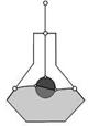
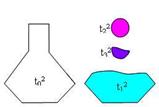
Fig. 3. (a) The pot filled with liquid model with nested cells and
(b) The 2D cells extracted
In this case the function ![]() takes the form
takes the form ![]() . Then the functions defining the 0D and 1D implicit cells
are defined on the basis of the description of the 2D cells as follows:
. Then the functions defining the 0D and 1D implicit cells
are defined on the basis of the description of the 2D cells as follows:
![]()
![]()
![]()
![]()
![]()
![]()
Note that each of the cells ![]() ,
, ![]() and
and ![]() consists of two
disconnected components. This does not contradict the implicit complex
definition and is useful in some applications (e.g., rendering). However, if it
is necessary to provide simple connectedness, then one can introduce additional
subdividing objects. The attributes here are defined though their RGB colour
components.
consists of two
disconnected components. This does not contradict the implicit complex
definition and is useful in some applications (e.g., rendering). However, if it
is necessary to provide simple connectedness, then one can introduce additional
subdividing objects. The attributes here are defined though their RGB colour
components.

Fig. 4. The pot filled with liquid: the 0D and 1D cells extracted
4.2. Discussion
Note the important distinctions between the proposed approach and the previously known frameworks for describing heterogeneous models. The models described in [11] also make use of subcomplexes derived from the basic cellular subdivision of the heterogeneous object. However, they first require the explicit building of the cellular subdivision of the modelling space and then use this to describe the subcomplexes representing the components of the object. In our framework the internal structure is described only for those components which really require such a detailed cellular representation. Other components are described using only the FRep of the corresponding point sets.
The models described in [6] make use of the topological stratification. Our framework does not need to exploit stratification-based structures since no strong topological restrictions on the subdomains that can be dimensionally heterogeneous non-manifolds are imposed. The main criterion for the choice of the subdomains is based on the specifics of their mathematical description. However, the proposed framework can be used to describe the topological stratification structures provided that the subdomains forming the object subdivision are manifolds with the topological homogeneity.
Also note that, as the above example demonstrates, nested cells are valid within our framework. This means that cells can intersect each other or lie inside other cells. For instance, in that example one part of the disc is inside the liquid and another is outside. To deal with such a model, we may either break the disk into two parts by removing the whole disk from the complex or subdividing the disk into two parts without deleting the whole disk. The latter case allows us to deal simultaneously both with the disk as a whole and with its parts and it is perfectly valid within the implicit complexes framework. Moreover, this allows for a flexible reconfiguration of the components of the model that promises interesting animation applications.
5. Rendering Implicit Complexes
Using the known rendering techniques such as polygonization and ray tracing, one can render any individual explicit or implicit cell. Below, we assume that the implicit complex contains cells with different opacity values. In the case of fully opaque cells, they can be rendered individually and combined together with the standard use of an appropriate Z-buffer. The example shown in Fig. 4 has been rendered with a conventional ray tracing algorithm extended to support trimmed implicit surfaces as 2D cells [12] and a Z-buffer. In the case of cells with different opacity values, a single Z-buffer is not enough, and direct visualization techniques (polygons and graphic hardware) can not be used. Indeed, not only a z-value has to be stored, but rather z intervals, in order to properly accumulate the opacity for a correct blending operation. Note that the order for rendering cells depends on their dimension. Therefore, to render implicit complexes, volume rendering techniques are also required, in addition to surface rendering techniques.
Explicit or implicit 1D and 2D cells are rendered first using traditional surface rendering techniques, as well as 3D explicit cells. Given a ray, all the z intersections have to be stored for each cell (a cell can intersect the ray several times). In the case of explicit 3D cells, z intervals are stored. It is sufficient to store only the set of z intervals for a 3D explicit cell, as inside such a cell opacity is constant by definition. At this stage of the rendering process, for the given ray several z values and z intervals along with the information that indicates the correspondence of the z value with its cell are stored.
Then, 3D implicit cells are rendered, depending on the stored values, with a volume rendering technique based on ray tracing. See, for instance, [4] for more details on general volume rendering. Using the previously stored information, z testing along the ray, one can determine if the current opacity and colour is accumulated depending only on the 3D implicit cell or whether the colour and opacity of another cell has to be used for the given point.
In the case of cells of a dimension lower or equal to 2, their colour and opacity are accumulated directly instead of the attribute values of the 3D implicit cell. In the case of 3D explicit cells, their attributes are accumulated along the stored z-interval. The z test along the ray and therefore the accumulation is performed until the traditional termination conditions have been met.
Fig. 5 shows an example of rendering of an implicit complex that contains cells of various dimensions and of various opacities. It also illustrates the theoretical example proposed in section 4, extended to 3D cells. The implicit 3D cells correspond to the grey cylinder and the pot-shape object. The colour of the object is based on Perlin’s noise function. The opacity varies along the vertical axis. Note that inside the pot there is a blue area (representing the liquid). This area, on the base of the constructive hypervolume model, is defined as a half-ellipsoid combined with a noise function. The 2D implicit cell is defined as a trimmed surface, namely an Escher’s spiral defined as a sphere surface trimmed by four swept solids. There are also 1D explicit cells shown in red that connect the 2D implicit cell and the 3D implicit cells (i.e., the cylinder). Note that the trimmed implicit surface intersects the 3D cell representing liquid as it is allowed in our model
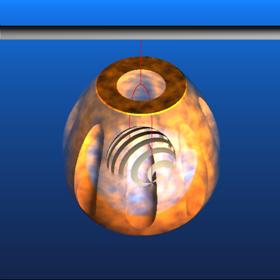
Fig. 5. Rendering an implicit complex composed of cells
of different dimension and semi-opaque cells.
6. Conclusions
Implicit complexes make it possible to combine a cellular representation and a constructive function representation into a uniform model. In this paper, we have described the theoretical framework and the practical techniques of construction and rendering such models. The general structure of an implicit complex and attachment operations were presented and illustrated. The general algorithm for rendering of implicit complexes including opaque and semi-transparent cells of arbitrary dimensions was proposed and illustrated.
Future work directions include the development of specific operations applicable to entire implicit complexes, an extension of the model to time-dependent implicit complexes, and further development of the multidimensional version of the model and its applications, and implementation of a specialized modelling language
References
[1] V. Adzhiev,
[2] Heterogeneous Objects Modelling and Applications, Collection of Papers on Foundations and Practice, Lecture Notes in Computer Science, vol. 4889, Eds. Pasko A., Adzhiev V., Comninos P., 2008, 285 p.
[3] T. Kunii (1999) Valid computational shape modeling: design and implementation, International Journal of Shape Modeling, vol. 5, No. 2, pp. 123-133.
[4] B. Lichtenbelt, R. Crane and
[5] W. S. Massey (1967), Algebraic topology: An introduction, Harcourt, Brace&World.
[6] A. Middleditch , C. Reade, A. Gomes (2000), Point-sets and cell structures relevant to computer aided design, Int. Journal of Shape Modeling, vol. 6, No. 2, pp. 175-205.
[7] K. Ohmori, T. Kunii (2001), Shape modeling using homotopy, In Proc. Int. Conf. on Shape Modeling and Applications, IEEE Computer Society, pp. 126-133.
[8] A. Paoluzzi, F. Bernardini, C. Cattani, V. Ferrucci (1993), Dimension-independent modeling with simplicial complexes. ACM TOG, vol. 12, No. 1, pp. 56-102.
[9] A. Pasko, V. Adzhiev, A. Sourin, V. Savchenko (1995), Function representation in geometric modeling: concepts, implementation and applications, The Visual Computer, vol. 11, No. 8, pp. 429-446.
[10] A. Pasko, V. Adzhiev, B. Schmitt, C. Schlick (2001), Constructive hypervolume modeling, Graphical Models, vol. 63, No. 6, pp. 413-442.
[11] J. Rossignac, M. O’Connor (1989), SGC: A dimension independent model for pointsets with internal structures and incomplete boundaries, In Geometric modeling for product engineering, ed. by M. Wozny, J. Turner, K. Preiss, pp. 145-180.
[12] B. Schmitt, A. Pasko, G. Pasko, T.
Kunii (2004), Rendering
trimmed implicit surfaces and curves, In Proc. Afrigraph 2004,