The paper deals with the problems concerning the representation and description of the dynamics of a smooth surface with a boundary at a given velocity field. An implicit representation of the surface is used with the help of the "closest point" method based on specifying a surface as a set of projections of points of space from some neighborhood of the surface onto the surface itself. Non-structured three-dimensional meshes that are not adapted to the surface geometry are used for the mesh representation of the domain containing the surface and for approximating the projection operator.

The problems of simulation of a surface during its motion in a given velocity field, computation the surface local bases at its interior points and at the boundary, and integration and differentiation of the functions defined on the surface are considered. A detailed description of the corresponding algorithms and the results of their testing are presented. The software used to visualize the calculation data is briefly described. The method of representation of data of modeling considered in this work not only makes it possible to use it effectively in computational algorithms, but it is also convenient for visual representation, which enables to understand better the dynamics of the process of crack development.

Keywords: surface evolution, the closest point method, unstructured meshes.

1. Introduction

The necessity of modelling of the dynamics of the surface with a boundary in a given velocity field arises in various problems of mathematical modelling and the computer graphics. The results of this study have been obtained in the course of developing the complex of computational algorithms for the problem of simulatio the dynamics of a large-scale hydraulic fracture of a oil ot gas reservoir.

The hydraulic fracturing is one of the most commonly used methods increasing oil recovery applied in the development of oil and gas fields. The essence of the fracturing technology consists in pumping a special liquid nto the oil reservoir to create an artificial crack with a length of ~100 m, height of ~10 m, and an average opening of ~5--10 mm. As a result, an artificial channel is created that is connected with a well and has a large inflow area and a high permeability (by orders of magnitude greater than the one of the oil reservoir). This provides a significant increase in the inflow of the formation fluid to the well. Engineering aspects of the technology are considered, for example, in [1, 2].

Physical and mathematical description of the crack dynamics in the course of its development in hydraulic fracturing consists in solving a complex interrelated problem including the following equation systems:

· a system of poroelasticity equations describing the evolution of stress-strain state of the formation and the fluid pressure fields in it during the development of the crack;

· equations of fluid flow in the crack;

· mechanical conditions for the development of the crack determining the direction of its development at each point of its front;

· dynamic interface conditions between the pressure field in the crack and in the formation defined on the lateral surfaces of the crack as well as kinematic conditions connecting the crack opening and the diaplacement of the formation.

In such a description, the geometrical model of the crack is a smooth surface with a movable boundary. The development of effective and reliable numerical methods for solving this problems includes the creation of a method for representing the median surface of the crack in a discrete problem taking into account the following:

· the change in the geometry of the median surface of the crack during its evolution is a priori unknown and is determined successively in the course of solving the complete interrelated problem;

· on the median surface of the crack, the equation of the lubricating layer describing the fluid flow in the crack and, indirectly, the crack evolution dynamics is solved;

· the complete problem is conjugate, so it is necessary to have a representation of the geometry of the crack which would make it possible to transfer the information about the fields given at the crack to a three-dimensional region.

To describe the geometry of a surface with a moving boundary, many approaches are known, including polygonal models, a parametric representation, a point cloud representation, an implicit representation through a level set approach, etc. All of them are quite efficient in the case when the final task consists only in describing the dynamics of the change in the geometry of the surface, like in a number of computer graphics problems. However, not all of them can be used to solve the above formulated problem of hydraulic fracturing simulation.

Among the known methods, the closest-point projection method was chosen as the most preferable. The motivation of this choice is primarily that there are known and well developed methods for solving differential equations on surfaces within the framework of this approach (see [3, 4, 5, 6]), and the surface representation method itself is well adapted for using it in conjunction with the X-FEM method to calculate the stress-strain state of the medium in the vicinity of the crack.

However, most of the works devoted to this method are associated with its application to the analysis of stationary surfaces or dynamic surfaces, but without a boundary. In this paper we propose an effective method for calculating the evolution of surfaces with a moving boundary; we consider the problems of representation, integration, and differentiation of functions defined on this surface, as well as the methods for calculating its local geometric properties, in particular, the construction of orthogonal bases at interior and boundary points of the surface.

It should be also noted that in most works on modeling the development of cracks with the help of the extended finite element method [7, 8, 9], the geometrical model of the crack is constructed using the level set method (see [10, 11]). Then, the surface with the boundary is given by a pair of scalar functions φ (x, t), ψ (x, t) defined in space such that

(1)

where t is time.

In other words, at a fixed time t, the surface is defined as a part of the level surface of the zero function bounded by the isosurface of the function . To carry out the calculations, it is convenient for the functions , to be the sign distances defined in some small neighborhood Ω of the surface F. The motion of the boundary of the surface is given by the velocity field describing the evolution of the functions , . For the recalculation of the functions , , the equations of Hamilton-Jacobi type are applied. The main disadvantage of this method is the complexity of its implementation: for example, to describe the evolution of a surface, an agreed solution of ten different Hamilton-Jacobi equations is required with respect to the functions and , ensuring, among other things, the orthogonality of their gradients, the properties of sign distances, etc. [7, 8, 9].

An alternative approach, somewhat similar to that used in this work, is described in [12]. The surface in this approach is defined by means of so-called "vector level sets", representing a pair of functions, the first of which is the operator projecting a point onto the surface in the sense of the nearest distance, and the second one determines the orientation of the surface. At the same time, the described approach uses a polygonal representation of the surface which is used for constructing the projection operators. During the evolution of the surface, its polygonal representation is updated first, and then, it is used to construct the projection operators and level functions.

In contrast to this approach, the present paper does not use the polygonal representation of the surface, and the values of projection operators in the course of its evolution are calculated directly. In this case, the surface itself and the level surfaces defining it can be reconstructed locally, if necessary. In this sense, the approach proposed in this paper and based on the closest- point projection method (CPPM) is more flexible and, in effect, it is close to the methods of representing surfaces as "point cloud surfaces" (see, for example, [ 15]).

Despite the fact that the algorithms presented in the paper were developed for solving a specific applied problem, they are universal and can be used to solve a wide range of problems related to the calculation and visualization of the dynamics of surfaces with a boundary.

In order to visualize the simulation results, the computer code FrontView developed at KIAM RAS is used in the work. Its main purpose is. "fast" visualization of large-volume data set on dynamic surfaces, which are described by unstructured triangular meshes.

The above described applied problem of evolution of the formation crack requires considering a complex coupled three-dimensional system of partial differential equations. The unknown fields are three-dimensional or two-dimensional, defined on the median surface of the fracture. The solution of the problem is also the evolution of the fracture itself, which is described as a smooth surface with a boundary in the considered problem statement. In general, the distribution of the properties of the medium containing the crack is three-dimensional. Therefore, a complete qualitative and quantitative analysis of the results of modeling is impossible without effective means of visualization. A set of existing means for visualization and analysis of modeling results, which would be suitable without additional adaptation to analysing the evolution of surfaces with a boundary is limited. For this reason, the approaches considered in this paper for describing the evolution of a surface with a boundary are of interest in itself in the context of problems of representation and visualization of modeling data.

2. CPP Method

Let us consider the basic concepts of the closest point method. A rigorous mathematical justification of this method is given in [13].

Let us consider a smooth surface with a boundary embedded in the three-dimensional space . Here and in what follows, the term "smooth" will mean that the set is an image of a smooth mapping of a bounded closed subdomain of the two-dimensional plane into the three-dimensional space . We will assume that the used mappings have any required number of derivatives. We also assume that the surface F is entirely located inside the spatial domain .

Let us suppose that for an arbitrary , is the closest point to it on the surface :

Here and below, the Euclidean norms are used.

The point will be called the projection of the point onto the surface in the sense of the shortest distance; the corresponding projection operator will be denoted by ,

The operator is vector-valued; it maps the domain onto the surface considered as a subset of . In the case that the surface and its boundary are smooth and the domain is "sufficiently small", the operator is uniquely defined, i.e., each point of is uniquely projected onto a single point on the surface.

If for the surface we can define the signed distance function (i.e., is an oriented surface without a boundary), then for the operator the following representation holds:

It can be shown that the projections operator uniquely describes the surface as a set of its fixed points:

It should be noted that this method of description is quite general. It allows one to describe the geometry of a surface with a boundary and without a boundary, nonorientable manifolds or manifolds of codimension greater than one (i.e., curves (codimension is equal to 2) and points (codimension is equal to 3), and also the union of objects of different codimension.

Further, it will be necessary to distinguish the points of that are projected into the interior points of or onto its boundary . With this purpose, let us consider the auxiliary operator which we define as [4]:

(2)

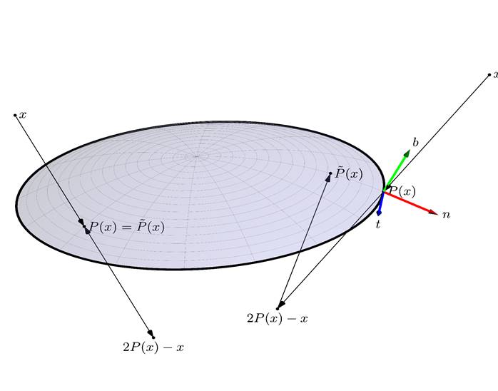
Fig. 1. Definition of operators and .

It follows from the geometrical consideration (see Fig. 1) that for the points whose projections belong to the boundary of the surface,

(3)

while for the points whose projections belong to the interior points of , the values of the projectors and coincide:

(4)

Together with the above presented method of describing the surface , we will need a way of representation of the functions defined on this surface. Due to the fact that there are no local coordinates on the surface , it is convenient to use the "implicit" way of their representation. Namely, a function on the surface will be defined as a trace on it of a function defined in the domain .

The extension of the function given on the surface to the domain can be constructed in various ways. A convenient and subsequently used method is its extension with the help of the operator . Namely, for an arbitrary function u given on the surface, its continuation in is defined as:

Thus, the constructed continuation is constant along the segments connecting a point of and its projection. This fact allows us to calculate the derivatives of a function on the surface in a convenient way, as well as differential operators of higher order (see below in this section).

It should be noted that for an arbitrary function in that is constant in the direction of the normal to , we have [13]:

where is the surface gradient (see [14]). Similarly, for an arbitrary smooth vector field in tangent to the surface :

Then, by virtue of the properties of the projector and the extension operator , we have:

Since the completion of is constant along directions normal to the surface, the vector field is tangent to . This implies that

where is the Beltrami-Laplace operator (the "surface" Laplace operator, [14]). Analogous extensions can also be constructed for more complicated elliptic operators of divergent type, see [3, 13].

3. Model of Surface Evolution

Above, we outlined the basic ideas of the closest point method with respect to a stationary surface. Let us formulate the problem of the surface evolution.

Let us designate time by t; the surface under consideration at time t by . We assume that for, the condition is satisfied. In other words, the family of surfaces corresponding to greater moments of time is contained within the surface corresponding to any greater moment of time. Or, which is the same, the surface can evolve only by moving its boundary. This situation corresponds to the specifics of the problem being solved, namely, the development of the median surface of the crack during the growth of the latter.

We will assume that:

• at each moment t within the interval under consideration, the surface is entirely contained inside the domain ;

• the evolution of the surface is "smooth", i.e, the surface at each moment of time can be smoothly and mutually unambiguously mapped onto, for example, a disc of unit radius in . In particular, in the course of evolution, self-intersections should not appear in , etc.

In this case, the family of surfaces can be represented as a union of the initial surface and the trace of the "motion" of its curvilinear boundary:

where is the movable boundary of the surface at time .

In what follows, we assume that a vector velocity , is defined on the line describing its evolution at each moment of time. Thus, the motion of a point of the boundary is described by equation

(5)

We assume that the velocity field is a smooth function of the point at each fixed time t and for each fixed (Lagrangian) point of the boundary is a smooth function of time.

At each moment of time, we will describe the surface with the help of the projection operator of the closest point. The construction of an algorithm for computing this operator (more precisely, its approximations) at each moment of time with its known value at the previous moments of time and a given velocity will be considered below.

4. Discrete Model of the Surface

Suppose that in a domain containing a surface , a computational mesh composed of tetrahedral cells is defined. The resulting triangulation will be considered regular (i.e., the intersection of two different tetrahedra can be an empty set, a mesh node, its boundary, or its face). We denote the corresponding discrete domain by . It is assumed that the mesh is sufficiently fine so that the characteristic mesh step is much smaller than the radii of the principal curvatures of the surface and the radius of the curvature of its boundary.

Let us denote the set of mesh nodes by , , and is the number of mesh nodes. We assign a basic function to each node of the mesh. In the simplest case, continuous piecewise-linear basis functions can be used for which , where is the Kronecker symbol, and the cells of the mesh are continued linearly.

In the discrete case, the projection operator is given by its values at the mesh nodes. To calculate the projection operator at an arbitrary point in the domain, the above introduced system of basis functions is used. If is an arbitrary point of the domain , is the tetrahedron in which it is located, is its barycentric coordinates with respect to the vertices of the tetrahedron , then the projection of the point is the point

The constructed approximations of the projector allow us to construct in a natural way the approximations of the projection in accordance with (2).

Now, let be the set of all nodes of the mesh. Define its subsets , , , corresponding to the nodes projected into the interior points of the surface and its boundary, respectively:

(6)

where is a small real parameter of the algorithm

Obviously, in the course of the surface evolution, the set can only increase (by inclusion). In other words, for we have:

This allows, in particular, as the surface moves, to update information at each next time step of the discrete sampling only for the nodes from the set .

5. Algorithm for Calculating the Surface Evolution

In this section, we consider the algorithm for recalculating the discrete sampling of the projector in the course of the surface evolution.

The general idea of the algorithm is as follows: first, according to the known information, the coordinates of the projection points of the mesh nodes from the set are calculated. Then, these points are shifted in a given direction in accordance with a given boundary speed and a given time step value. The resulting points belong to the new position of the front, but the vector connecting the original node of the spatial mesh and the new position of the boundary point is not the projection vector of the closest point. Therefore, the approximations of the projector are corrected.

Then, we will assume that the surface evolves on the time interval . We introduce on this interval a computational mesh with steps , ,

where is the number of mesh nodes.

At the initial time , the approximation of the projector is assumed to be known. We also assume that during the time interval , the surface remains inside the mesh domain .

The complete algorithm for constructing the discrete operator at time for given parameters of the method and the known approximation is presented in the scheme of Algorithm 1.

The input data of the algorithm are the discrete sampling of the projector at a time and the sets and . As a result of application of the algorithm, the values of input data are replaced by the corresponding values of output data at time .

The parameters of the method are the values , , and . The parameter determines the conditionality of the projection of a point on the segment and the accuracy of the projection computation,

where determines the radius of the sphere bounding the region in which the points are searched for in step 6 of algorithm 1. It is assumed that is sufficiently large as compared with the mesh spacing, but does not exceed the maximum distance from the point to its projection onto the boundary,

In the general case, it suffices to put . The parameter defines the threshold value that is used to determine whether the projection belongs to the boundary of the surface or to the set of its interior points. When calculating the value of (see step 5 of the algorithm), the same value of the parameter as that in (6) should be used.

1.	Input Data: Discrete representation of the surface at time : sets , , projector approximations , time step, algorithm parameters: , , , ..
2.	Set
3.	Calculate the new positions of all projections onto the boundary in accordance with approximation (5):
4.	Forall // For all nodes projecting onto the boundary
5.		Determine the closest to node from :
6.		Define (sub)set such that:
7.		if // Point is a projection onto the boundary of the surface.
8.			Set
9.		else // Point is not projection onto the boundary of the surface.
10.			Find such a point among the points in that the length of the is minimal:
11.			Set
12.		end if
		// Determine the projection of the point onto the segment :
13.		Set
14.		if // The point is projected onto the surface.
15.			Set
16.		else if // The point is projected onto the boundary.
17.			Set
18.		else if // The point is projected onto the surface.
19.			Set
20.		end if
21.	end forall
22.	Output data: a discrete representation of the surface at : the sets , , the projector approximations .

Algorithm 1. Calculation of the evolution of the projector .

6. Integration over the Surface

Let us consider the problem of integrating functions on the surfaces given by the "closest point" projector. Specifically, we will deal with the calculation of integrals of the form:

or, in a particular case, with the calculation of the area of the surface under consideration with a boundary:

Let us consider the discrete case. We assume, like it was made above, that the surface is located inside some mesh domain . Let be its boundary formed by the union of triangular faces :

where is the number of faces. With a known partition of the domain , the set of faces can be easily defined as the set of faces incident to one and only one tetrahedron of the triangulation.

Let us represent in the form of a union of three pairwise disjoint sets:

where consists of faces, all nodes of which are projected onto the front (i.e., they are elements of the set ); and are the sets of other faces; all the faces of the sets and lie on the same side of the surface.

We note that:

• all nodes of the faces from are projected onto the boundary of the surface. The areas of triangles whose vertices are the projections of the vertices of triangles from are negligible when the mesh spacing tends to zero;

• the projection operator (both continuous and discrete) bounded on the set is a surjection (mapping "onto") onto the surface ;

• In the case when a straight line passing through an arbitrary point on the surface and oriented by a unit normal to it intersects the boundaries of the set one at a time, then triangular meshes defined on generate triangular meshes on the surface . The nodes of these meshes are formed by the projections Vertices of triangles from , while two nodes of this mesh are considered to be connected by a boundary if the corresponding nodes in are connected to it.

To calculate the integrals of the functions defined on the surface, we will, in fact, use these meshes; in order to calculate the approximate value of the integral over a single triangle we will use the single-point quadrature formula.

In this case, there is no need to represent explicitly in the algorithm the described above meshes on the surface , since summation over triangles of such a mesh can be carried out in a cycle over all triangles forming the set . The contribution from the triangles belonging to the set will be vanishingly small at , while the contribution from the surfaces will be (asymptotically) doubled.

Next, if a straight line passing through an arbitrary point on the surface and oriented by the unit normal to it intersects the boundaries of the set more than once, the projections of the meshes will no longer form a correct mesh on , since the projections of the individual triangles can have a non-empty intersection. In this case, the above presented calculation scheme must be corrected. Namely, it is necessary to take into account the mutual orientation of the outer normal to the face and the directions of the projection, for example, of its center.

Thus, let us consider some face (triangle) , formed by mesh nodes , , and . Correspondingly, the fourth node of the tetrahedron will be denoted by . Then the normal to the face is given by the following expression:

where the sign «» denotes the vector product in . The direction of the normal can be determined from the mutual orientation of the calculated normal and the vector connecting the center of the face and its projection. Namely, the normal vector will be the outer normal vector if

In what follows, we will consider that this condition is satisfied.

Therefore, we come to the following expression for computing the surface integral:

where is some extension of the function g from the surface to the domain . If , then we have:

and the expression for the approximate calculation of the integral is simplified.

The factor «2» before the integral arises from the fact that the integral is calculated twice by traversing triangles from and from .

7. Calculation of Local Bases on a Surface and its Boundary

In the context of the considered applied problem, namely, the problem of modeling the evolution of a large-scale crack of hydraulic fracturing, it becomes necessary to calculate local vector bases at the boundary and on the surface and its neighborhood. In particular, this is required when using the extended finite element method (X-FEM) to calculate the stress-strain state in the host medium. This section considers this and allied problems.

Let us introduce another projection operator , which is a projection operator in the sense of the shortest distance to the boundary of the surface:

The operator is well-defined (in the sense of the uniqueness of the projection) in some sufficiently small neighborhood of the boundary of the surface . We denote the corresponding neighborhood by .

We assume that (a) and (b) the domain contains all the points of that are projected onto the boundary of the surface in the sense of criteria (3) and (4). Next, let be the subdomain of and domains consisting of the points that are projected onto the boundary of the surface (see Fig. 2).

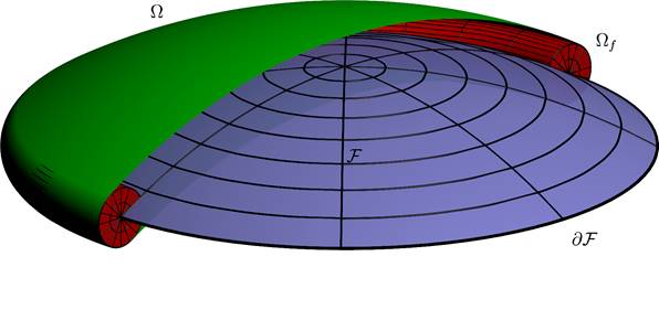
Fig. 2: Domains , , and

It follows from this that:

• In the subdomain all three operators , and are defined;

• The images of the operators and acting on the domain coincide with each other and with the set of points of the boundary of the surface.

If we denote the set of points of the set projected onto the boundary of the surface , then the set can be chosen in the form:

i.e, this set is obtained by "mirror" reflection of the set with respect to the surface boundary. The same algorithm can also be used to construct the domain in the discrete problem statement.

Let us consider the problem of constructing the local bases on the surface and its boundary.

At all points of the projections of the mesh nodes from the set , the vector of the unit normal to the surface can be defined as:

. (7)

The directions of the vectors for all the nodes of the mesh lying "on the same side" from the surface coincide with each other. In the case when the surface is "slightly curved", i.e., its radius of curvature is considerably larger than the diameter of the surface itself, the orientation of the surface can be uniquely determined by the choice (not depending on the point of the surface and the domain ) of the vector . In this case, for the mesh node , , the position of the node and the normal orientation can be determined by computing the sign of the scalar product .

Thefore, at all nodes of the set , the value of the approximation of the function of the sign distance to the surface can be restored:

At an arbitrary point of the domain projected onto the surface (but not at its boundary), the vector of the unit normal at the projection point and the value of the sign-distance function can be restored by interpolation. If are the barycentric coordinates of the point with respect to the tetrahedron in which it is located, then we have:

where are defined according to (7). Let us consider similar questions for the points whose projection lies at the boundary of the surface.

Let be a vector at the point of the boundary of the surface that is normal to its boundary and lies on the tangent plane of the surface. For an arbitrary point of the domain (the "tubular" neighborhood of the surface boundary), we define the approximation of the vector n at the projection point as:

It is obviously that this vector approximates the exact value of the normal vector with an accuracy . If the "diameter" of the tubular domain decreases linearly with computational mesh convergence (for example, the "diameter" of the domain is limited by a fixed number of elements of the mesh, then

The approximation of the vector tangent to the boundary of the surface at the point can be calculated as:

Finally, the vector , which is the normal to both the surface and its boundary, can be defined as:

The constructions presented above are illustrated in Fig. 1.

Thus, at each projection point, a local orthogonal basis of vectors can be constructed. The orientation of this basis can be determined if we know a "global" vector which specifies the orientation of the surface (see above) and does not depend on the point of the surface.

Such a basis allows us to introduce the local Cartesian and polar coordinates in each "section" of the tubular domain according to the rule:

where the function is defined everywhere except for the point , in accordance with:

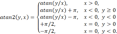
and returns the value of the polar angle of the vector in the basis .

The functions that define the surface and its boundary as null set (see (1)) can be reconstructed as:

Finally, it is possible to make a local reconstruction of the surface directly in the neighborhood of points on both the surface and its endge. To do this, one can use the methods developed when dealing with the representation of surfaces as a set of points belonging to them ("point cloud surfaces"), see, for example, [15].

8. Testing of algorithms

The developed algorithms for calculating the evolution of a surface with a boundary and integrating the functions defined on it were programmed in C ++ and Python for the GNU Linux OS. Below, the results of testing the implementations of these algorithms are presented. To visualize the results of calculations, the FrontView program was used. Its brief description is given in the corresponding section.

8.1. Disc in the uniform velocity field

As a first test, let us consider the problem of development of a plane surface, which is a trace of a disk of radius moving in a translation motion with a constant velocity. At the initial time, the surface is defined as a half of such a disk located in the region . The computational domain has the form of a parallelepiped with sides parallel to the coordinate axes. The disk plane is horizontal, its center at the initial moment of time coincides with the center of the lateral face of the computational domain. The velocity field specified at the boundary of the disk is assumed to be constant and homogeneous at all points of the boundary, , . Then, at time t, the center of the disk is located at the point . The surface is formed as a trace from the motion of the disk in the computational domain.

Direct calculations yield the following analytic expression for the projector P:

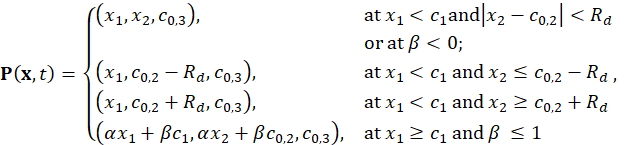
where , , , , are the Cartesian coordinates of the domain.

The time dependence of the crack area has the form:

8.2. Disk in the vortex velocity field

As a second test, let us consider a similar problem, in which, however, the surface is not flat. Like it was made above, we assume that at the initial moment of time, the surface is a half of a disk, however, now located on the surface of a cylinder with a given radius. In the course of evolution, the surface remains on the cylinder, "wound" on it along the section, the plane of which is perpendicular to the axis of the cylinder. The axis of the cylinder is parallel to the coordinate axis . The velocity field is vortex with an axis parallel to the axis . It is assumed that the vortex axis is on the right boundary of the computational domain and passes through the point . Then the velocity field has the form:

where is the distance from the point of space to the axis of the vortex, at which the velocity modulus is .

Let be the radius of the cylinder to which the surface belongs. We introduce the angular coordinate on the surface of the cylinder. Then, the coordinates of the points on the surface of the cylinder will have the form:

If at the initial moment of time the center of the disk along the -axis has the coordinate , then the equation of the surface boundary can be written in the parametric form as follows:

where is a parameter. In this case, the condition of projection onto the boundary (i.e., the condition of the minimum distance from the point of space to the boundary) can be written in the form:

Hence, the following equation is obtained with respect to the value of corresponding to the projection of a given point of space onto the curvilinear boundary of the surface:

In calculations, when constructing an exact solution, this equation is solved by Newton's method.

The analytical solution for the projector is:

where .

For the surface area, the following expression holds:

8.3. Results of testing.

In the testing process, we studied the dependence of the mean error in determining the projection at the end of the calculation at a given

where the summation is carried out over all nodes of the computational mesh and the error in determining the area

on the characteristic mesh spacing h.

It should be noted that the algorithm for calculating the evolution of the surface does not use any information about the mesh structure; its operation requires only information about coordinates of its nodes. At the same time, the information about the mesh structure is needed to calculate integrals of functions defined on the surface.

For the calculation, we used a mesh consisting of tetrahedra with a characteristic spacing , not adapted to the geometry of the surface. The test parameters had the values , for the case of a disk in a uniform velocity field and , , for a disk in a vortex velocity field.

In all calculations, the time step and the modeling time , .

Fig. 3 shows the phases of the evolution of the surface for the test named as "a disk in a homogeneous velocity field" which considers the evolution of a plane surface, which is a trace of a disk of a given radius moving with a constant velocity. The details of the test are described in section 8.1.

Fig. 4 demonstrates the animations corresponding to the "disk in the vortex speed field" test. The initial configuration of the surface is a disk on the surface of a cylinder. The velocity field is axisymmetric with the rotation axis coinciding with the axis of the cylinder. A detailed description of the test is given in Section 8.2. The left animation shows the evolution of the surface itself. The color indicates the error of the mesh approximation of the surface. On the right, one can see the animation of the evolution of the boundary of an unstructured tetrahedral mesh enclosing the surface with the boundary. The mesh shown in the animation is used to represent the surface by means of the closest point projection method. As the surface evolves, the tetrahedral mesh is being completed appropriately. A detailed description of the test is given in section 8.2. of the paper. The color indicates the error level of the mesh approximation of the surface.

The graphs in Fig. 5 show the dependence of the calculation error of the projector and the surface area during its evolution on the mesh spacing. It can be seen that the constructed algorithm has the order of convergence with respect to close to the second one.

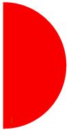
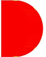
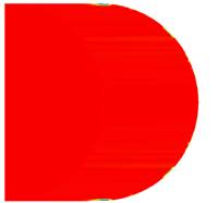
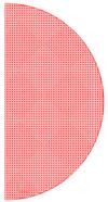
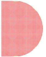
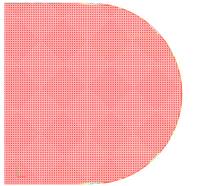
Fig. 3. Evolution of a disk in a homogeneous velocity field at , , the color indicates the level of the projection error on the interval

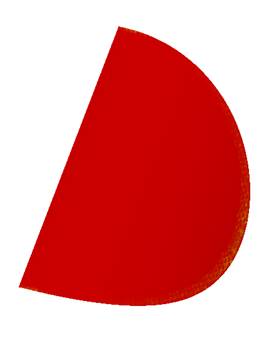
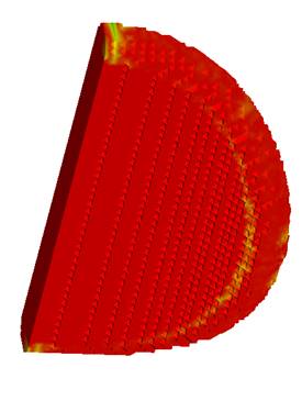
Fig. 4. Evolution of a disk in a vortex velocity field at , , the color indicates the level of the projection error on the interval


(а)	(b)

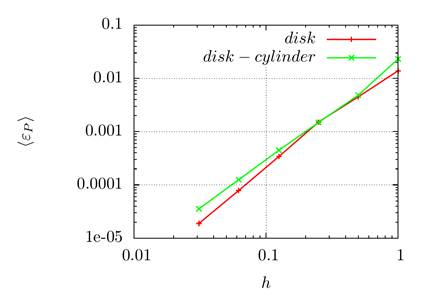
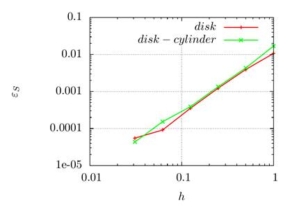
Fig. 5. Dependence of the errors and on the parameter for two test statements: a disc in an uniform velocity field ("disk" curves) and a disk in a vortex velocity field ("disk-cylinder" curves)

9. Visualizer FrontView

To visualize the results, the FrontView application was used. It was originally developed in Keldysh Institute of Applied Mathematics of the Russian Academy of Sciences by S.A. Khilkov (MIPT) in the process of solving the problem of seismic migration before summation in the asymptotic approximation. The main purpose of this program is a rapid visualization of a large amount of data set on dynamic surfaces represented as unstructured triangular meshes.

The FrontView application is developed under Linux OS in C ++ and Python languages using OpenGL libraries (www.opengl.com) and glm (http://glm.g-truc.net). To visualize data, the FrontView application uses its own binary data format; to organize the data recording, the user is provided with a header file in C ++.

To visualize time-dependent fields, the data is written into a single file in a frame-by-frame manner, the frames are sequentially located in the file. Each frame contains the instantaneous value of the visualized fields. Data related to different time points can be specified on different meshes. The data corresponding to one frame includes a triangular unstructured mesh in 3D-space---the coordinates of the vertices are a list of triples of indices that define triangular cells of the mesh. Each cell and each vertex of the mesh can be associated with additional information---an arbitrary (but the same for all cells) number of values in the float4 format. In this way, the data format allows one to store various scalar and vector fields on the mesh.

When working with the FrontView application, the user can navigate between frames, select viewing angles and zooming, activate the clipping planes, save a constructed image in various raster graphic formats. When mapping, four user-selectable data arrays are used: three arrays are displayed as the coordinates of the vertices of the triangles (by default, these are the coordinates of the vertices of the initial mesh), the fourth data array is displayed in color. This approach allows an efficient visualization of various projections of complex multidimensional functions. In the problem considered in this paper, both the coordinates of the vertices of the initial mesh and their projections onto the surface to be approximated were chosen as coordinates. Color, as a rule, indicates the error value.

The FrontView application interface consists of a window, in which the visualization is carried out, and a command-line interface. The transition between frames, changing viewing angles and zooming are possible with the help of both a mouse and hotkeys. The command-line interface uses the syntax of Python, calling the exec function to parse user commands. This allows one to configure flexibly the visualization parameters, create various data processing scripts, and perform batch processing (for example, using loops and other Python control constructs).

10. Conclusions

This paper has dealt with the problems related to the representation and calculation of the dynamics of surfaces with a boundary. To represent the surface, the "closest point" method was used. The problems of representation of functions on such surfaces and calculation of their differential characteristics are considered. A new algorithm for calculating the evolution of surfaces using a given velocity field and the algorithm for integrating the functions defined on a surface are proposed. In comparison with the methods traditionally used for such problems, which are based on the representation of a surface as a zero-level set of a given function, the constructed algorithm does not require solving the equations of Hamilton-Jacobi type and proves to be much simpler in implementation on unstructured meshes. The results of numerical calculations demonstrated the appropriate accuracy and efficiency of the proposed algorithms for applications. The description of the FrontView program used to visualize the calculation data is given. The method of representation of the data of modeling considered in this work not only allows one to use it effectively in computational algorithms, but it is also convenient for the visual representation, which makes it possible to better understand the dynamics of the process of crack development.

Acknowledgements

This work was supported by the Russian Science Foundation, project no. 15-11-00021.

References

1. Ekonomides M., Olini R., and Val’ko P. Unifitsirovannyi dizain gidrorazryva plasta. Ot teorii k practike [Unified Design of Hydraulic Fracturing. From Theory to Practice]. Institute of Computer Science, 2007, p.236.

2. Salimov V.G., Ibragimov N.G., Nasybullin A.V., and Salimov O.V. Gidravlicheskii razryv karbonatnyh plastov [Hydraulic Fracturing of Carbonaceous Formations]. Neftyanoe Hozyaistvo, 2013, p. 471.

3. Ruuth S.J., Merriman B.M. A simple embedding method for solving partial differential equations on surfaces. J. Comput. Phys., 227 (2008), pp. 1943–1961.

4. Macdonald C.B., Brandman J., Ruuth S.J. Solving eigenvalue problems on curved surfaces using the Closest Point Method. J. Comput. Phys., 230 (2011), pp. 7944–7956.

5. Macdonald C.B., Ruuth S.J. Level set equations on surfaces via the Closest Point Method. J. Sci. Comput., 35 (2008), pp. 219–240.

6. Macdonald C.B., Ruuth S.J. The implicit Closest Point Method for the numerical solution of partial differential equations on surfaces. SIAM J. Sci. Comput., 31 (2009), pp. 4330–4350.

7. Stolarska M., Chopp D., Moes N., Belytschko T. Modelling crack growth by level sets in the extended finite element method. Int. J. Numer. Meth. Engng. 2001; 51:943–960.

8. Moes, N., Gravouil, A., Belytschko, T. Non-planar 3D crack growth by the extended fiite element and level sets—Part I: Mechanical model. Int. J. Numer. Meth. Engng 2002; 53:2549–2568 (DOI: 10.1002/nme.429)

9. Gravouil, A., Moës, N., Belytschko, T. Non-planar 3D crack growth by the extended finite element and level sets—Part II: Level set update. Int. J. Numer. Meth. Engng. V. 53, 2002. pp. 2569–2586. DOI: 10.1002/nme.430.

10. Osher, S. J., Fedkiw, R.P. Level Set Methods and Dynamic Implicit Surfaces. Springer-Verlag. ISBN 0-387-95482-1. 2002.

11. Sethian, J. A. Level Set Methods and Fast Marching Methods : Evolving Interfaces in Computational Geometry, Fluid Mechanics, Computer Vision, and Materials Science. Cambridge University Press. ISBN 0-521-64557-3. 1999.

12. Ventura G., Budyn, E., Belytschko T. Vector level sets for description of propagating cracks in finite elements. Int. J. Numer. Meth. Engng 2003; 58:1571–1592 (DOI: 10.1002/nme.829).

13. März T., Macdonald C.B. Calculus on surfaces with general closest point functions. SIAM J. Numer. Anal., Vol. 50, No. 6, pp. 3303–3328.

14. Dubrovin B.A., Novikov S.P., and Fomenko A.T. Sovremennaya geometriya: metody I prilozheniya [Modern Geometry: methods and applications]. Nauka, 1986, p. 760.

15. Berger M., Tagliasacchi A., Seversky L., Alliez, P., Levine, J., Sharf, A., Silva, C. State of the Art in Surface Reconstruction from Point Clouds. EUROGRAPHICS 2014 / S. Lefebvre and M. Spagnuolo. STAR –– State of The Art Report, 2014.