FUZZY SURFACE VISUALIZATION USING HSL COLOUR MODEL
Jan Caha(http://orcid.org/0000-0003-0165-0606)1, Alena Vondráková(http://orcid.org/0000-0002-7450-467X)2
1Department of Regional Development and Public Administration, Mendel University in Brno, Brno, Czech Republic
2Department of Geoinformatics, Faculty of Science, Palacký University in Olomouc, Olomouc, Czech Republic
Email: jan.caha@mendelu.cz, alena.vondrakova@upol.cz
Contents
6. Possible further extensions of the proposed approach
6.1. Visualization of another information from fuzzy number
6.2. Visualization of vector data
6.3. Visualization of another type of uncertainty
Appendix A: Software - Fuzzy Data Visualizer
Abstract
Fuzzy surfaces are surface models that account for the uncertainty that originates either in data or from user's uncertainty about the interpolation settings. So far, fuzzy surfaces have been visualized as 3D projections, profiles or as separate visualizations of three surfaces that show minimal, modal and maximal estimated value. Unfortunately, neither of these approaches towards fuzzy surface visualization is quite suitable for practical application. 3D projections and profiles manage to capture only part of the surface and three separate visualization are extremely challenging for users. In ideal case the user needs to obtain complete information (including uncertainty) about whole surface in the simplest visualization possible. As a result of these issues, a new method for fuzzy surface visualization is proposed. The method utilizes hue saturation lightness (HSL) colour model to depict the most important values of the predicted fuzzy surface. The method combines properties of the set of fuzzy numbers, that form the fuzzy surface, with properties of colour defined in HSL colour model. The resulting visualization utilizes continuous two-dimensional gamut to visualize the fuzzy surface. In cartography, however, the continuous gamuts are often consider as needlessly challenging for users (to obtain the correct information); so as a simplification a discrete variant of the two dimensional gamut is provided as well. The variant of visualization utilizing the discrete gamut is designed to be as customizable as possible, so that it is possible to adapt the visualization (in terms of complexity) for various groups of users from experts to non-experts. The proposed approaches are defined in terms of equations that allow visualization of arbitrary fuzzy surface with high level of visualization customization. The visualization method is presented on practical case study. A simple software, that allows testing of the proposed visualization, is provided as an appendix of the paper.
Keywords: fuzzy surface, uncertainty, visualization, HSL, geovisualization
1. Introduction
One of the main issues associated with spatial interpolation is the fact that the resulting visualizations often provide users with a false impression that the visible results are entirely precise while the opposite is true (Skeels, Lee, Smith, Robertson 2010). The predicted data contain uncertainty that may originate from data imprecision, vagueness or randomness. Another source of uncertainty is the interpolation method itself. Some interpolation methods like kriging even provide the estimation of uncertainty that arises directly from the prediction process. For kriging, this uncertainty is presented in a form of the standard deviation of prediction error (Hengl 2003). The interpolation method can also be affected by uncertainty as a result of user’s uncertainty regarding parameters settings for the interpolation (Loquin, Dubois 2010). However, for the decision making that commonly follows the spatial prediction, it is not important where in the previous process uncertainty originates but how it affects the results. (Edwards, Nelson 2001) state that data validity is the key to making credible decisions. As a consequence, it is necessary from the visualization point of view to pass on to the user not only the information about predicted values but also the information about certainty (or uncertainty) of the prediction (Skeels, Lee, Smith, Robertson 2010).
The presented research focuses on visualization of fuzzy surfaces. Fuzzy surfaces are special type of surfaces that incorporate uncertainty of data (Diamond 1989; Santos, Lodwick, Neumaier 2002; Waelder 2007), epistemic uncertainty of user regarding the settings of interpolation (Bardossy, Bogardi, Kelly 1990; Loquin, Dubois 2010) or both (Loquin, Dubois 2010; Soltani-Mohammadi 2015). Unlike the statistical approaches of representing uncertainty of surface, such as the one presented by (Hengl 2003), the uncertainty of fuzzy surface does not have to be symmetrical. This fact renders visualization methods like so called “whitening” (Hengl 2003) unsuitable for visualization of fuzzy surfaces. The problem of visualization is often neglected when dealing with fuzzy surfaces, mainly because most of the research focuses on construction of fuzzy surfaces (Caha, Vondráková 2014).
There has been some research regarding visualization of fuzzy information (Jiang 1996; Bastin, Fisher, Wood 2002; Pham, Brown 2005; Park, Park 2010) with the focus mainly on fuzzy sets and fuzzy logic systems. Unfortunately, the results obtained from the mentioned studies cannot be applied to visualization of fuzzy surfaces as the type of uncertainty differs significantly amongst those topics.
The main aim of this research is to provide a method for visualization that will allow a representation of the predicted value along with its uncertainty. According to the categorization of spatial uncertainty visualizations provided by (Kinkeldey, MacEachren, Schiewe 2014), the presented method falls in into categories of explicit (directly displaying uncertainty), intrinsic (altering existing symbology), visually integral (uncertainty cannot be separated from the data), coincident (both data and uncertainty are represented in one view) and static (no dynamic elements) representations. The organization of the rest of the paper is following section Theoretical background provides necessary information about fuzzy surfaces and HSL (hue saturation lightness) colour model. Section Proposed approach describes the procedure for fuzzy surface visualization. A practical example of the proposed approach is shown in section Case study. In the last section, several conclusions are drawn.
2. Theoretical background
This chapter summarizes the necessary concepts of fuzzy surfaces and the HSL colour model. Fuzzy surfaces are a particular type of surface that represent not only the surface but also its uncertainty. The uncertainty of the surface is modelled with the utilization of fuzzy numbers which are also described in this section. A thorough explanation of these concepts is essential for the visualization approach that is explained in section Proposed approach.
2.1. Fuzzy numbers
A fuzzy number is a unique case of a fuzzy set that represents the uncertain, imprecise or ill-know variable (Dubois, Prade 1979). Fuzzy numbers are used to model values that cannot be specified precisely, but there are indications of the most likely correct value as well as extreme values that provide limits. For example, value ’approximately two’ can be modelled as a fuzzy number with the most likely value 2 and limits 1 and 3. Given the uncertain description the user can only conclude that the vague value is higher than 1, lower than 3 and the most likely correct representation is 2. Such vague description of number is an ideal starting point for modelling using fuzzy numbers.
In the same way as a fuzzy set a fuzzy number ![]() is
described by a membership function which is defined by mapping:
is
described by a membership function which is defined by mapping:
![]()
that indicates that element ![]() of universe
of universe ![]() has the membership
value
has the membership
value ![]() from
the interval
from
the interval ![]() (Zadeh 1965). Element
(Zadeh 1965). Element ![]() with
with ![]() does
not belong to the fuzzy set, element
does
not belong to the fuzzy set, element ![]() with
with ![]() belongs
to the set completely. Other values from the interval
belongs
to the set completely. Other values from the interval ![]() denote partial
membership.
denote partial
membership.
In order to be a fuzzy number, the fuzzy set ![]() has
to satisfy several conditions (Hanss 2005). The universe on which the set is
defined should be real numbers
has
to satisfy several conditions (Hanss 2005). The universe on which the set is
defined should be real numbers ![]() . The
height of the fuzzy set according to
. The
height of the fuzzy set according to
![]()
must be equal to 1. So that there is one and exactly one ![]() with full membership
to the set
with full membership
to the set ![]() . This
value is called peak or modal value of a fuzzy number. Sometimes fuzzy numbers
that have more than one
. This
value is called peak or modal value of a fuzzy number. Sometimes fuzzy numbers
that have more than one ![]() with
with ![]() are
also considered as fuzzy numbers. However, for the purpose of this research
only fuzzy numbers with one
are
also considered as fuzzy numbers. However, for the purpose of this research
only fuzzy numbers with one ![]() with
with ![]() are
considered.
are
considered.
Next condition is that the fuzzy set also has to be convex, which it is, if the condition
![]()
is satisfied. The support of the fuzzy set has to bounded.
The last condition is that the membership function ![]() must
be at least piecewise continuous. If the fuzzy set satisfy all those conditions
it can be treated as a fuzzy number, which means that it can be used for
further calculations (Hanss 2005).
must
be at least piecewise continuous. If the fuzzy set satisfy all those conditions
it can be treated as a fuzzy number, which means that it can be used for
further calculations (Hanss 2005).
Every fuzzy number consist of three values that are of
specific interest to the decision maker. These values are the minimal, modal
(or peak) and maximal value of the fuzzy number. Using these three values a
fuzzy number ![]() can
be described as triplet
can
be described as triplet ![]() (Fig.
1). This triplet can also be a definition of a triangular fuzzy numbers (Hanss
2005; Santos, Lodwick, Neumaier 2002). From the decision-making perspective, it
is important to note that the fuzzy number does not have to be symmetrical,
which means that
(Fig.
1). This triplet can also be a definition of a triangular fuzzy numbers (Hanss
2005; Santos, Lodwick, Neumaier 2002). From the decision-making perspective, it
is important to note that the fuzzy number does not have to be symmetrical,
which means that ![]() (Fig.
1).
(Fig.
1).
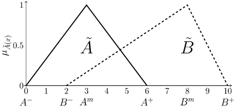
Fig. 1. Example of symmetrical fuzzy number ![]() and
nonsymmetrical fuzzy number
and
nonsymmetrical fuzzy number ![]() with
their minimal, modal and maximal values.
with
their minimal, modal and maximal values.
2.2. Fuzzy surfaces
The fuzzy surface is a surface that has for every coordinate
![]() the
height defined not as a precise number
the
height defined not as a precise number ![]() but
has as a fuzzy number
but
has as a fuzzy number ![]() (Santos,
Lodwick, Neumaier 2002). The fuzzy number
(Santos,
Lodwick, Neumaier 2002). The fuzzy number ![]() located
at
located
at ![]() describes all the possible values that
the surface can have at this location. If the surface is described is modelled
as a grid, then each its cell is a fuzzy number. Fuzzy model of surface
naturally captures uncertainty associated with the spatial prediction.
describes all the possible values that
the surface can have at this location. If the surface is described is modelled
as a grid, then each its cell is a fuzzy number. Fuzzy model of surface
naturally captures uncertainty associated with the spatial prediction.
Fuzzy surfaces were first introduced almost concurrently by (Diamond 1989) and (Bardossy, Bogardi, Kelly 1990). Each of those authors utilized different approach towards the construction of fuzzy surfaces. While (Diamond 1989) proposed interpolation of uncertain data (modelled as fuzzy numbers), (Bardossy, Bogardi, Kelly 1990) propose interpolation of precise data by krigging method with uncertain parameters (again modelled as fuzzy numbers). Although these approaches provide the same result (fuzzy surface), they are internally very distinct with each of them focused on a different type of uncertainty in the interpolation process. Later subsequent approaches for fuzzy surface interpolation were proposed (Santos, Lodwick, Neumaier 2002; Lodwick, Santos 2003; Waelder 2007) and the approach suggested by (Bardossy, Bogardi, Kelly 1990) was further developed by (Loquin, Dubois 2010). Until recently there were no software tools available that would be able to carry out the computation necessary to construct fuzzy surface. However, that changed with the introduction of FuzzyKrig (Soltani-Mohammadi 2015).
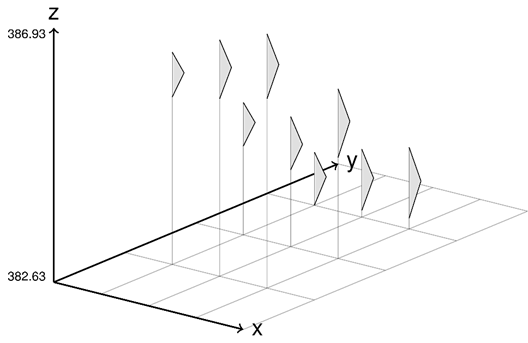
Fig. 2. Example of 3D representation of small fuzzy
surface (![]() points).
points).
There is still relatively little attention directed towards
visualization of fuzzy surfaces in the existing literature. Usually, profiles
and 3D projections (Fig. 2) of fuzzy surface (Bardossy, Bogardi, Kelly 1990;
Diamond 1989; Lodwick, Santos 2003; Loquin, Dubois 2010; Santos, Lodwick,
Neumaier 2002) or three separate surfaces (Fig. 3), representing values of ![]() and
and ![]() (Caha,
Marek, Dvorský 2015; Soltani-Mohammadi 2015), are visualized; however,
neither of these are quite suitable for user perception. Profiles and 3D
representations only capture part of the fuzzy surface and the separate
visualization for each significant value makes it complicated for user to
assess the differences. Classic example of three separate surfaces is in Fig.
3; such visualization makes it really hard for the user to assess the
differences amongst the surfaces and to identify the amount of uncertainty in
specific locations. Thus, a new approach is necessary that will allow more
suitable visualization of fuzzy surface.
(Caha,
Marek, Dvorský 2015; Soltani-Mohammadi 2015), are visualized; however,
neither of these are quite suitable for user perception. Profiles and 3D
representations only capture part of the fuzzy surface and the separate
visualization for each significant value makes it complicated for user to
assess the differences. Classic example of three separate surfaces is in Fig.
3; such visualization makes it really hard for the user to assess the
differences amongst the surfaces and to identify the amount of uncertainty in
specific locations. Thus, a new approach is necessary that will allow more
suitable visualization of fuzzy surface.
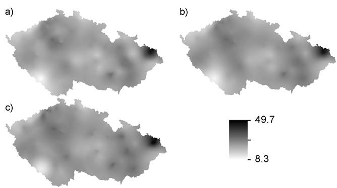
Fig. 3. Example of fuzzy surface visualization using 3
surfaces. The dataset shows concentration of ![]() in
in ![]() .
Variant a) represents
.
Variant a) represents ![]() , b)
, b) ![]() and
c)
and
c) ![]() .
.
3. HSL Colour Model
The typical colour systems integrated into cartography and GIS software are RGB (red green blue), HSV (hue saturation value), HSB (hue saturation brightness), HSL (hue saturation lightness) and CMYK (cyan magenta yellow black) (Brewer, Hatchard, Harrower 2003). In general, colours represent a hugely important area of cartography. Bertin (Bertin 2010) classified colour value and colour hue as a part of seven initial visual variables of a cartographic design. (MacEachren 2004) later extended this systematisation, and the importance of colour schemes is still emphasized. Colour models used for spatial visualization and cartographic design preferences are in the vast majority based on the request for final processing (Dent, Torguson, Hodler 2009). For printed maps model CMYK is principally used, for digital maps mostly RGB or HSB models are used.
(Joblove, Greenberg 1978) firstly described the HSL (hue
saturation lightness) colour model. As other relative colour models (e.g. HSV
(hue saturation value), HSB (hue saturation brightness)), it is based on the
tiling of RGB cube so that the black colour is at the origin with white
directly above it. The colours red, yellow, green, magenta, blue and cyan are mapped
on a circle using interval ![]() . Hue
values starts with red starting at
. Hue
values starts with red starting at ![]() 1.
The saturation describes the distance
of the colour from the main (black - white) axis, and lightness specifies the
amount of white present in the resulting colour. Both saturation and lightness
take values from the interval
1.
The saturation describes the distance
of the colour from the main (black - white) axis, and lightness specifies the
amount of white present in the resulting colour. Both saturation and lightness
take values from the interval ![]() . The
model can be visualized as a cylinder (Fig. 4).
. The
model can be visualized as a cylinder (Fig. 4).
Fig. 4. Cylindrical model of HSL (left) and bicone variant that shows chroma instead of saturation (right). (based on: (Joblove, Greenberg 1978))
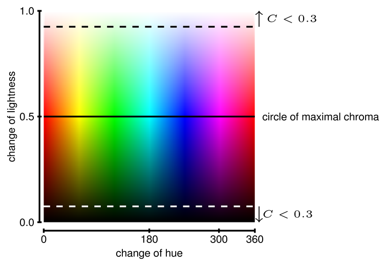
Fig. 5. Surface of the cylindrical model of HSL with colours with chrome lower than 0.3 shown. Note colours between hue values 300-360, that cannot be used to avoid confusion with colours close to value 0.
Important characteristics of colour in HSL model is its chroma, which is colourfulness relative to the white colour with similar lightness. If chroma is used instead of saturation when plotting the model, the cylinder becomes bicone (Fig. 4). This variant of visualization better captures the amount of possible colours for different values of lightness. Because if lightness is equal to 1 or 0 the colour is always white or black without relation to hue. The chroma of colour in HSL is calculated as:
![]()
where ![]() is a value of chroma,
is a value of chroma, ![]() is lightness and
is lightness and ![]() denotes saturation.
Low values of
denotes saturation.
Low values of ![]() suggest that the colour is on black -
grey - white scale and its hue will be hard to determine. Fig. 5 shows the
surface of the cylindrical model from Fig. 4 with parts of the surface with low
values (smaller than 0.3) of chroma denoted. It is apparent from this
visualization that it would be impossible for the user to determine correct hue
of colour with small values of
suggest that the colour is on black -
grey - white scale and its hue will be hard to determine. Fig. 5 shows the
surface of the cylindrical model from Fig. 4 with parts of the surface with low
values (smaller than 0.3) of chroma denoted. It is apparent from this
visualization that it would be impossible for the user to determine correct hue
of colour with small values of ![]() . Quantifying this limit is directly
dependent on the ability of map user to distinguish colors. Based on Eq. (4) it
can be determined that ranges of lightness
. Quantifying this limit is directly
dependent on the ability of map user to distinguish colors. Based on Eq. (4) it
can be determined that ranges of lightness ![]() and
and ![]() should
be omitted from the set of colours to provide distinguishable colours. Fig. 5
also illustrates the problem with the circular nature of hue that was mentioned
previously.
should
be omitted from the set of colours to provide distinguishable colours. Fig. 5
also illustrates the problem with the circular nature of hue that was mentioned
previously.
The transformation from HSL colour model to RGB colour model as well as conversions to other models are in detail described by (Joblove, Greenberg 1978).
4. Proposed approach
The proposed approach is based and highly influenced by the
work (Zehner, Watanabe, Kolditz 2010) and (Hengl 2003), who presented
visualization methods for data with uncertainty based on changes of saturation,
brightness and/or intensity. Suppose that there is a set of fuzzy numbers ![]() (e.g.
set of fuzzy numbers that forms fuzzy surface) each with its set of important
values
(e.g.
set of fuzzy numbers that forms fuzzy surface) each with its set of important
values ![]() . For
each fuzzy number values of uncertainty between modal and both limit values can
be calculated as:
. For
each fuzzy number values of uncertainty between modal and both limit values can
be calculated as:
![]()
![]()
Where ![]() is
the magnitude of the uncertainty between the modal and minimal value of a fuzzy
number and
is
the magnitude of the uncertainty between the modal and minimal value of a fuzzy
number and ![]() is a
magnitude of uncertainty between maximal and modal value. Along with the modal
(or peak) value of fuzzy number these two numbers describe the magnitude of
uncertainty related to a fuzzy number (Fig. 6).
is a
magnitude of uncertainty between maximal and modal value. Along with the modal
(or peak) value of fuzzy number these two numbers describe the magnitude of
uncertainty related to a fuzzy number (Fig. 6).
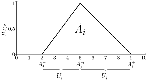
Fig. 6. Fuzzy number ![]() with
its important points
with
its important points ![]() and
magnitudes of uncertainty
and
magnitudes of uncertainty ![]() and
and ![]() .
.
From the set of fuzzy numbers mentioned previously ![]() and
uncertainty values
and
uncertainty values ![]() and
and ![]() four
values that will be important for our visualization technique can be
calculated:
four
values that will be important for our visualization technique can be
calculated:
![]()
![]()
![]()
![]()
The values ![]() and
and ![]() )
describe the range of modal values of all the fuzzy numbers from the set. The
values
)
describe the range of modal values of all the fuzzy numbers from the set. The
values ![]() ,
, ![]() show
the maximal magnitudes of uncertainty from modal value towards minimal and
maximal values respectively.
show
the maximal magnitudes of uncertainty from modal value towards minimal and
maximal values respectively.
In the proposed approach two components of HSL model are
used to visualize the modal value of fuzzy surface and magnitudes of
uncertainty to produce two maps that allow the user to observe the modal values
as well as deviations from this value towards both sides. The modal value of a
fuzzy number is associated with hue; ![]() is
related to the difference of lightness from the mean value towards zero and
is
related to the difference of lightness from the mean value towards zero and ![]() is
connected with the difference of lightness towards one. The value of saturation
is considered as fixed with value 1.
is
connected with the difference of lightness towards one. The value of saturation
is considered as fixed with value 1.
To make the proposed approach as flexible as possible, it is
not expected that whole ranges of hues or lightness have to be used in the
visualization. Rather a user can specify ranges of hue and lightness that
he/she wishes to use. Based on his decision variables ![]() ,
, ![]() ,
, ![]() ,
, ![]() that
describe ranges of hue and lightness are introduced. These values have to
fulfil simple rules in order to provide meaningful results:
that
describe ranges of hue and lightness are introduced. These values have to
fulfil simple rules in order to provide meaningful results: ![]() and
and ![]() ,
where
,
where ![]() denotes
a middle value of
denotes
a middle value of ![]() .
.
For every fuzzy number ![]() from
the set of fuzzy numbers
from
the set of fuzzy numbers ![]() we
can calculate:
we
can calculate:
![]()
![]()
![]()
The values of ![]() and
and ![]() denotes
lightness for the two images. The example of the two-dimensional legend and two
fuzzy numbers is shown in Fig. 7.
denotes
lightness for the two images. The example of the two-dimensional legend and two
fuzzy numbers is shown in Fig. 7.
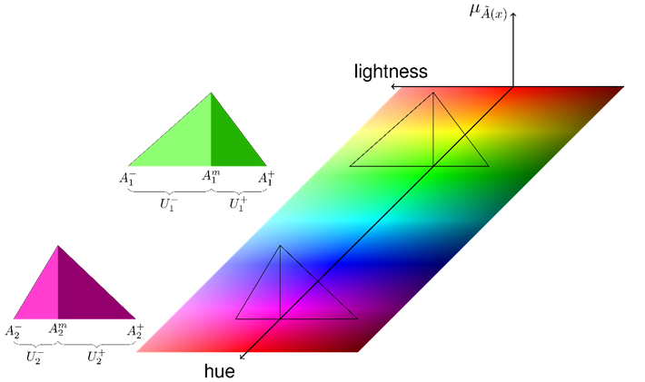
Fig. 7. An example of two fuzzy numbers on two-dimensional legend with the critical colour values shown.
For the two resulting maps, the colour for the map showing
the magnitude of uncertainty towards smaller values is defined in HSL model as ![]() . The
map showing the magnitude of uncertainty towards high values the colour is
defined as
. The
map showing the magnitude of uncertainty towards high values the colour is
defined as ![]() . The
value of
. The
value of ![]() is the same for both models. Fig. 7
shows an example of two fuzzy numbers with the legend and colours of minimal
and maximal uncertainty values presented by lightness change.
is the same for both models. Fig. 7
shows an example of two fuzzy numbers with the legend and colours of minimal
and maximal uncertainty values presented by lightness change.
5. Discrete colour scheme
In the theory of cartographic visualisation, it is needed to deal with user aspects of the final colour scheme (MacEachren, Robinson, Hopper, Gardner, Murray, Gahegan, Hetzler 2005). For many users, it is difficult to perceive a variety of information in a smooth transition gamut (Vondráková 2013). Concomitant use of multi-parameter changes colours makes this situation even more difficult for a significant part of users. To ensure proper perception and subsequent interpretation of the data it is reasonable to discretize the legend into the interval scheme (Vondráková, Caha 2014). According to the scale, purpose and target user groups of visualization it is possible to select an appropriate number of intervals for the map. The interval colour scheme is often used in thematic cartography, for example in choropleth maps. Therefore, this approach is the application of methods of thematic cartography, which are commonly used for its utility and efficiency (Dent, Torguson, Hodler 2009).
The method for visualization of fuzzy numbers described
above that utilizes continuous scales of hue and lightness is computationally
simple. However, such scale is not very suitable for users. The two-dimensional
legend as described above might be too complicated, and thus, a simplification
is necessary to make more comprehensible for the user. Such simplification can
be done by categorization of both hue and lightness into ![]() and
and ![]() categories, which
limits the number of used colours on the map to
categories, which
limits the number of used colours on the map to ![]() . For simplification
of the visualization,
. For simplification
of the visualization, ![]() is required to be an even number.
is required to be an even number.
The example of this discretization is shown in Fig. 8. In
this figure, an interval ![]() is
divided into
is
divided into ![]() categories. The colour for each category
is determined from the continuous legend as midpoints of the intervals. The
first and last intervals get values of hue
categories. The colour for each category
is determined from the continuous legend as midpoints of the intervals. The
first and last intervals get values of hue ![]() , so
that whole range of hue is used. The resulting legend includes relatively
distinct colours, especially when compared to a continuous legend. As a result,
the information from the map is much easier to read for the user.
, so
that whole range of hue is used. The resulting legend includes relatively
distinct colours, especially when compared to a continuous legend. As a result,
the information from the map is much easier to read for the user.
The specific values of hue for each interval are obtained as:
![]()
In this equation ![]() denotes the index of interval with first
interval having index
denotes the index of interval with first
interval having index ![]() and thus its hue is \(minH\). Every
modal value of fuzzy numbers is then categorized into respective category and
the relevant hue value is assigned.
and thus its hue is \(minH\). Every
modal value of fuzzy numbers is then categorized into respective category and
the relevant hue value is assigned.
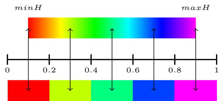
Fig. 8. The process of determination of hues for interval legend.
The identical process can be done for the values of lightness,
resulting in discretized legend for uncertainty of fuzzy numbers. As mentioned,
the number of categories for lightness denoted as ![]() , is required to be an
even number. That way it is easier to define the categories with
, is required to be an
even number. That way it is easier to define the categories with ![]() below
the
below
the ![]() and the
same number of categories above
and the
same number of categories above ![]() . The
values of
. The
values of ![]() for categories are calculated as:
for categories are calculated as:
![]()
In this equation, ![]() denotes the index of the interval with
the first interval having index
denotes the index of the interval with
the first interval having index ![]() . In the same way as hue is categorized
in the description above, the values of
. In the same way as hue is categorized
in the description above, the values of ![]() and
and ![]() are
categorized to obtain the value of lightness.
are
categorized to obtain the value of lightness.
Graphical representation of this process is in Fig. 9. The combination of discretized lightness and hue values results in the two-dimensional legend categorical legend.
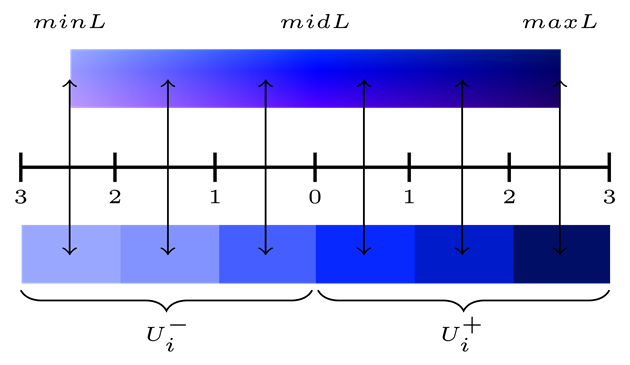
Fig. 9. The process of determination of lightness values for interval legend.
An example of how lightness is determined for three fuzzy
numbers with identical modal value is shown in Fig. 10. The figure shows lightness
divided into six intervals. Intervals with negative values on ![]() axis show deviation
towards smaller values while the positive values indicate uncertainty towards
higher values. The final colours used in visualization for the particular fuzzy
number is determined by the intervals in which the values of
axis show deviation
towards smaller values while the positive values indicate uncertainty towards
higher values. The final colours used in visualization for the particular fuzzy
number is determined by the intervals in which the values of ![]() and
and ![]() fall
in.
fall
in.
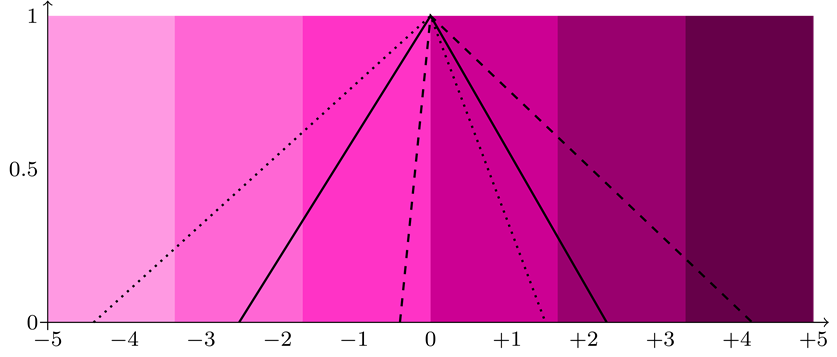
Fig. 10. Three fuzzy numbers with equal modal value and with varying amounts of uncertainty shown on a lightness scale.
6. Possible further extensions of the proposed approach
The utilization of proposed approach can be done in three main directions. These directions are a) visualization of another information from fuzzy number, b) visualization of vector data, c) visualization of another type of uncertainty.
6.1. Visualization of another information from fuzzy number
The presented approach is focused on visualization of
triangular fuzzy numbers and uses three most important values of a triangular
fuzzy number to do so. The reason for using this type of fuzzy number is that
is the most commonly implemented in practical applications (Hanss 2005) and it
is also the most illustrative example for users. However, there is an
interesting potential to visualize either other types of fuzzy numbers (i.e.
Gaussian or trapezoidal) as well as other parts of fuzzy numbers. In order to
do so, we need to introduce so-called ![]() -cut
which is an interval
-cut
which is an interval ![]() with
specified membership value
with
specified membership value ![]() . For more details about
. For more details about ![]() -cuts see (Zadeh 1965)
and (Hanss 2005). The proposed approach utilizes the whole range of fuzzy
numbers by the use of its limit values. However, by substituting
-cuts see (Zadeh 1965)
and (Hanss 2005). The proposed approach utilizes the whole range of fuzzy
numbers by the use of its limit values. However, by substituting ![]() with
with ![]() in
Eq. (5) and by
in
Eq. (5) and by ![]() with
with ![]() in
Eq. (6) the differences can be calculated to another
in
Eq. (6) the differences can be calculated to another ![]() -cut. This allows the
visualization of the only portion of uncertainty. Such approach can be
favourable in certain decision-making situations. It also allows users to
assess differences among various levels of uncertainty. In chapter Fuzzy
numbers it is mentioned that only fuzzy numbers containing one
-cut. This allows the
visualization of the only portion of uncertainty. Such approach can be
favourable in certain decision-making situations. It also allows users to
assess differences among various levels of uncertainty. In chapter Fuzzy
numbers it is mentioned that only fuzzy numbers containing one ![]() with
with ![]() are
considered. Fuzzy numbers with more than one
are
considered. Fuzzy numbers with more than one ![]() that satisfy this
condition also exist in the literature (see (Hanss 2005)). Such fuzzy numbers
do not have the single value of
that satisfy this
condition also exist in the literature (see (Hanss 2005)). Such fuzzy numbers
do not have the single value of ![]() .
These can also be visualized using the proposed approach in case that their
modal value is simplified into a single value. For example using this equation:
.
These can also be visualized using the proposed approach in case that their
modal value is simplified into a single value. For example using this equation:
![]()
In this situation, the midpoint of \(\alpha\)-cut with value 1 (the core of fuzzy number) is used as the main reference value.
6.2. Visualization of vector data
The proposed approach focuses on visualization of surface data represented as raster. The nature of calculations necessary to obtain both colours for visualization is general enough so that it can be calculated from a vector dataset as well. In the beginning of section Proposed approach there is a mention about a set of fuzzy number. This set can be obtained from various types of data. This property allows simple extension of this visualization approach to other types of data. For example, polygons with values of attribute predicted in a form of fuzzy number can be visualized using the proposed approach.
6.3. Visualization of another type of uncertainty
The proposed approach focuses on visualization of uncertainty modelled by fuzzy numbers. In theory, another uncertainty theories can be used as well. The uncertain value has to have some kind of modal or most likely value as well as lower and upper limit. If those three values can be determined than the proposed method of visualization can be used. However, the proposed approach might not be the best case when all the uncertain values are symmetrical around the modal value. In such case, there is no need to visualized three parameters because two parameters (modal value and uncertainty) would be enough.
7. Case Study
The fuzzy surface used for the visualization in the case
study is taken from (Caha, Marek, Dvorský 2015)2. The fuzzy surface
represents the monthly average of concentrations of ![]() air
pollutant in Czech Republic for October 2013. The values of concentration are
in in
air
pollutant in Czech Republic for October 2013. The values of concentration are
in in ![]() . The
data from 182 locations are used to construct fuzzy surface by interpolation
with fuzzy variogram (Fig. 11). The method used to calculate the fuzzy surface
was proposed by (Loquin, Dubois 2010) and the detailed process of calculation
is described by (Caha, Marek, Dvorský 2015). A FuzzyKrig tool
(Soltani-Mohammadi 2015) can be used to calculate fuzzy surface based on the
described data and fuzzy variogram.
. The
data from 182 locations are used to construct fuzzy surface by interpolation
with fuzzy variogram (Fig. 11). The method used to calculate the fuzzy surface
was proposed by (Loquin, Dubois 2010) and the detailed process of calculation
is described by (Caha, Marek, Dvorský 2015). A FuzzyKrig tool
(Soltani-Mohammadi 2015) can be used to calculate fuzzy surface based on the
described data and fuzzy variogram.
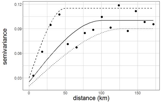
Fig. 11. Fuzzy variogram used in interpolate fuzzy surface. (source: (Caha, Marek, Dvorský 2015))
The fuzzy surface is represent using proposed approach with
continuous scale (Fig. 12) as well as using discrete colour scheme (Fig. 13). For
this case study values of ![]() ),
), ![]() ,
, ![]() and
and ![]() were
selected for definition of colour ranges according to Eqs. (11,12, 13). From
the set of fuzzy numbers the following statistics:
were
selected for definition of colour ranges according to Eqs. (11,12, 13). From
the set of fuzzy numbers the following statistics:
![]()
![]()
![]()
![]()
are obtained and used to construct the visualization. The
resulting maps are visualized in Fig. 12 using continuous legend with hue limit
values - ![]() ,
, ![]() and
lightness limit values -
and
lightness limit values - ![]() and
and ![]() .
.
Fig. 13 shows visualization using discrete colour scheme with the same limit values as continuous scale and 5 categories of hue and 10 categories of lightness. The number of categories in the case study was selected based on expert opinion as a compromise between number of categories and amount of information in the resulting visualization. The number of classes is selected with respect to the type of users and main aim of the map. For example if the users are not well acquainted to the uncertainty problematic the number of lightness categories can be reduced to four. For more experienced users the values around ten should be comprehensible. The continuous scale quite possible suitable only for experts and for interactive visualizations that would allow users to query the data directly through interaction. For the visual assessment of surface uncertainty the discreate colour scheme should be preferred.
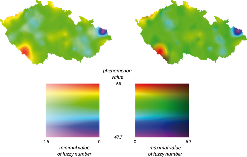
Fig. 12. Visualization with applications of whitening and darkening approach — continuous colour scale.
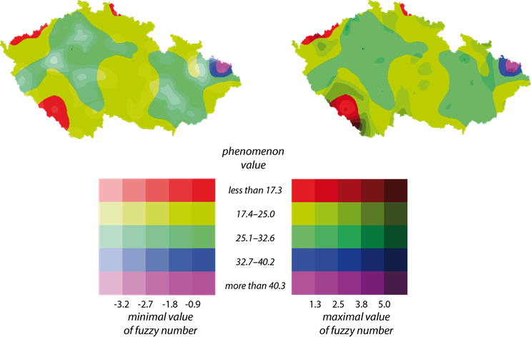
Fig. 13. Visualization with applications of whitening and darkening approach — interval colour scale.
Both visualizations (Figs. 12, 13) show the nonsymmetrical
character of uncertainty in the example. Clearly there are more significant
deviations towards ![]() than
than ![]() . The differences
almost make impression that there is no uncertainty towards higher values,
especially on the continuous scale (Fig. 12).
. The differences
almost make impression that there is no uncertainty towards higher values,
especially on the continuous scale (Fig. 12).
8. Conclusion
The presented research focuses on the fuzzy surfaces visualization with emhpasis on the asymmetry of fuzzy numbers. Hue allows the map user to estimate the modal (most possibly true) value of the fuzzy surface, and whiteness and darkness provide him the estimation of minimal and maximal value (deviations from the modal value caused by uncertainty). Information perception of fuzzy surfaces visualizations made by internal graphic variables HSL model should be more suitable, than the most commonly used approaches used so far (profiles, 3D visualizations and separate representation of important values).
The general perception of geovisualization is significantly affected by a particular user, his/hers knowledge, skills and other characteristics, but the main aim of the researcher is to provide as accurate information as possible, which is enabled by the suitable methods of visualization.
Even though the presented visualization method is shown on the fuzzy surface, it is defined universally, so that it can be used for other types of uncertainty visualization. The proposed approach can also be applied for example to statistical data by replacing modal value of fuzzy number by mean value and using differences amongst mean and minimum and maximum as the two measures of uncertainty. Further research should focus on testing users attitude towards the proposed visualization method by objective means such as eye-tracking.
Acknowledgement
The authors gratefully acknowledge the support by the Operational Program Education for Competitiveness - European Social Fund (projects CZ.1.07/2.3.00/20.0170 and CZ.1.07/2.2.00/28.0078 of the Ministry of Education, Youth and Sports of the Czech Republic).
Appendix A: Software - Fuzzy Data Visualizer
For practical testing of the proposed approach of visualization of fuzzy data a software was programmed in C# language. The software is called Fuzzy Data Visualizer and allows construction of two dimensional legend using both continuous and discretized scale of the legend, as described in section Proposed approach. The graphical user interface of the legend design is shown in Fig. 14.
The legend can be created independently or it can be based on fuzzy dataset provided as a “.csv” file. An example file is provided with the software for testing purposes. The data after being loaded into the software are interactively visualized in the tab “Data Visualization” using the currently specified legend. The Data Visualization part of the graphical user interface is shown in Fig. 15.
The described software is freely available from the https://github.com/JanCaha/FuzzyDataVisualizer as an appendix to this paper.
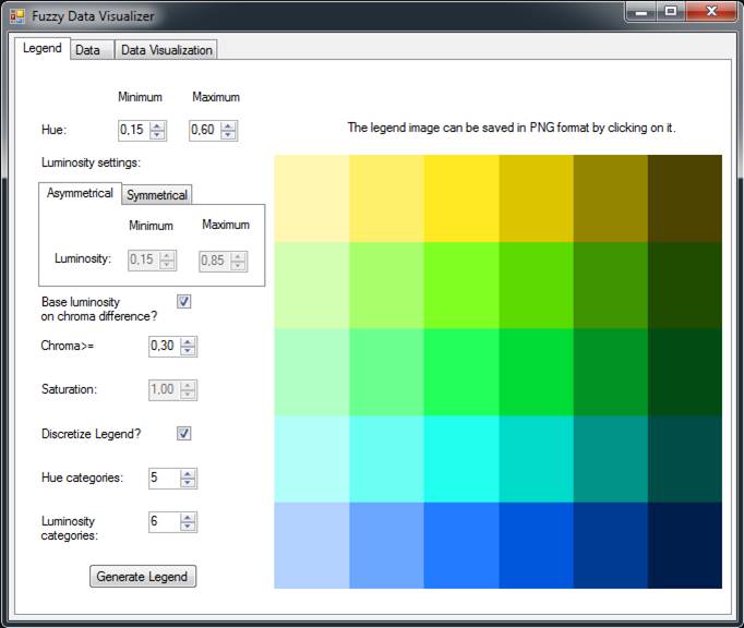
Fig. 14. Graphical user interface of Fuzzy Data Visualized -- legend design.
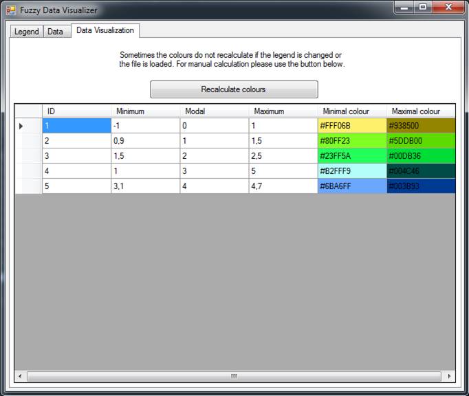
Fig. 15. Graphical user interface of Fuzzy Data Visualized — data interactive visualization.
References
1. Bardossy A., Bogardi I. And Kelly W. E. Kriging with imprecise (fuzzy) variograms. II: Application. Mathematical Geology. January 1990. Vol. 22, no. 1, p. 81–94.
2. Bastin L., Fisher P.F. And Wood J. Visualizing uncertainty in multi-spectral remotely sensed imagery. Computers and Geosciences. 2002. Vol. 28, no. 3, p. 337–350. DOI 10.1016/S0098-3004(01)00051-6.
3. Bertin J. Semiology of graphics: Diagrams, networks, maps. 1st ed. Redlands, CA.: ESRI Press.
4. Brewer C.A., Hatchard G.W. And Harrower M.A. ColorBrewer in print: A catalog of color schemes for maps. Cartography and Geographic Information Society. 2003. Vol. 30, p. 5–32.
5. Caha J. And Vondráková A. Visualizing relevant uncertain information for decision making: Fuzzy surface case study [online]. 2014. Available from: http://cognitivegiscience.psu.edu/uncertainty2014/papers/caha_fuzzy.pdf
6. Caha J., Marek L. And Dvorský J. Predicting PM10 Concentrations Using Fuzzy Kriging. In : Hybrid artificial intelligent systems se - 31. Springer International Publishing. p. 371–381. Lecture notes in computer science.
7. Dent B.D., Torguson J.S. and Hodler T.W. Cartography: Thematic map design. 6th ed. Thomas Timp.
8. Diamond P. Fuzzy Kriging. Fuzzy Sets and Systems. 1989. Vol. 33, no. 3, p. 315–332.
9. Dubois D. and Prade H. Fuzzy real algebra: Some results. Fuzzy Sets and Systems1. 1979. Vol. 2, p. 327–348.
10. Edwards Ld and Nelson Es. Visualizing data certainty: A case study using graduated circle maps. Cartographic Perspectives. 2001. No. 38, p. 19–36.
11. Hanss M. Applied Fuzzy Arithmetic: An Introduction with Engineering Applications. Berlin ; New York : Springer-Verlag.
12. Hengl T. Visualisation of uncertainty using the HSI colour model: computations with colours. In: Proceedings of the 7th international conference on geocomputation. Southampton. 2003. p. 8.
13. Jiang B. Fuzzy Overlay Analysis and Visualization in Geographic Information Systems. PhD Thesis. University of Utrecht.
14. Joblove G.H. and Greenberg D. Color spaces for computer graphics. Computer Graphics. 1978. Vol. 12, no. 3, p. 20–25.
15. Kinkeldey C., Maceachren A.M. and Schiewe J. How to assess visual communication of uncertainty? A systematic review of geospatial uncertainty visualisation user studies. Cartographic Journal. 2014. Vol. 51, no. 4, p. 372–386.
16. Lodwick W.A. and Santos J. Constructing consistent fuzzy surfaces from fuzzy data. Fuzzy Sets and Systems. 2003. Vol. 135, no. 2, p. 259–277.
17. Loquin K. and Dubois D. Kriging with Ill-Known Variogram and Data. In : Scalable uncertainty management. Springer Berlin / Heidelberg. p. 219–235. Lecture notes in computer science.
18. Maceachren A.M. How maps work, representation, visualization, and design. 1st ed. New York. : The Guilford Press.
19. Maceachren A.M., Robinson A., Hopper S., Gardner S., Murray R., Gahegan M. and Hetzler E. Visualizing Geospatial Information Uncertainty: What We Know and What We Need to Know. Cartography and Geographic Information Science. 2005. Vol. 32, no. 3, p. 139–160.
20. Park Y. and Park J. Disk diagram: An interactive visualization technique of fuzzy set operations for the analysis of fuzzy data. Information Visualization. 2010. Vol. 9, no. 3, p. 220–232. DOI 10.1057/ivs.2010.3.
21. Pham B. and Brown R. Visualisation of fuzzy systems: requirements, techniques and framework. Future Generation Computer Systems-the International Journal of Grid Computing and Escience. 2005. Vol. 21, no. 7, p. 1199–1212. DOI 10.1016/j.future.2004.04.007.
22. Santos J., Lodwick W.A. and Neumaier A. A New Approach to Incorporate Uncertainty in Terrain Modeling. In : Geographic information science. Springer Berlin Heidelberg. p. 291–299. Lecture notes in computer science.
23. Skeels M., Lee B., Smith G. and Robertson G.G. Revealing uncertainty for information visualization. Information Visualization. 2010. Vol. 9, no. December 2008, p. 70–81. DOI 10.1057/ivs.2009.1.
24. Soltani-Mohammadi S. FuzzyKrig: a comprehensive matlab toolbox for geostatistical estimation of imprecise information. Earth Science Informatics. 2015.
25. Vondráková A. Non-technological aspects of map production. In : In 13th international multidisciplinary scientific geoconference and expo, sgem 2013. Albena. 2013. p. 813–820.
26. Vondráková A. and Caha J. Visualization of fuzzy surfaces. In : International multidisciplinary scientific geoconference surveying geology and mining ecology management, sgem. Sofia : STEF92 Technology Ltd. 2014. p. 1069–1076.
27. Waelder O. An application of the fuzzy theory in surface interpolation and surface deformation analysis. Fuzzy Sets and Systems. 2007. Vol. 158, no. 14, p. 1535–1545.
28. Zadeh L.A. Fuzzy Sets. Information and Control. 1965. Vol. 8, no. 3, p. 338–353.
29. Zehner B., Watanabe N. and Kolditz O. Visualization of gridded scalar data with uncertainty in geosciences. Computers & Geosciences. October 2010. Vol. 36, no. 10, p. 1268–1275.
- Due to the circular nature of
hue, it is worth to note both values
 and
and
 are red. That means that hues after
cyan are gain by mixing the cyan with red (Fig. 5). As this may pose
problems for cartographic visualization, we recommend using only the
interval
are red. That means that hues after
cyan are gain by mixing the cyan with red (Fig. 5). As this may pose
problems for cartographic visualization, we recommend using only the
interval  for practical applications. (Hengl
2003) suggests the similar solution of this problem.↩
for practical applications. (Hengl
2003) suggests the similar solution of this problem.↩ - The dataset used in this paper is available from https://github.com/JanCaha/FuzzySurface.↩