METRICS FOR MEASURING COMPLEXITY OF GEOMETRIC MODELS
A.A. Globa1, M. Donn2, O.A. Ulchitskiy3
1Research Fellow Deakin University, Melbourne, Australia;
2Victoria University of Wellington, New Zealand;
3Nosov Magnitogorsk State Technical University, Magnitogorsk, Russia;
globalnaya@gmail.com, michael.donn@vuw.ac.nz, o.ulchitsky@magtu.ru
Contents
2.0 Speed of Algorithmic Modelling
3.0 Outcome 3D Model Complexity Evaluation, Point System
3.1 Basic elements (Geometrical Complexity)
3.2 Composition Space (Dimensional complexity)
3.3 Arithmetic of Shapes (Shape Grammars)
3.4 Transformations (Shape Grammars)
3.5 Number of Elements (Components)
Abstract
This study considers the practical methodology for measuring the level of complexity of geometric patterns in architecture. Criteria for forming the metric complexity of the models include geometric, combinatorial and spatial categories. The study also used methodology 'Grammar Form' (Shape Grammar), based on figures arithmetic and logical analysis of the forming mechanisms. This article explains the theory and methodology measurement of geometric complexity of models and illustrates the practical application of this analysis on the fifty-parametrically generated 3D models.
The study has been developed as a part of wider research, which focuses on parametric modelling and ways to support the use of parametric design: by decreasing the number of programming difficulties, and increasing the explored solution space, programming efficiency, the degree of the algorithms’ sophistication and the speed of algorithmic modelling (level of model complexity). Research has included a series of parametric modelling workshops. In order to provide experimental data for this research, participants developed and submitted practical assignments and filled in online questionnaires. This paper explains the ‘step by step’ methodology for measuring the complexity of geometric models and illustrates practical applications of this analysis for the modelling outcomes from the first workshop.
Keywords: model complexity, architectural model, parametric modeling, shape grammars, computer-aided design, geometric model analysis.
1.0 Experimental Framework
The study was organised in the form of two-day parametric modeling workshops with a capacity of thirty attendees. The workshop offered an introduction to algorithmic computational design using Grasshopper [Grasshopper 3d, 2013] for Rhinoceros [Rhino3d, 2012]. The course taught 3D modelling fundamentals and the advantages of using parametric modelling. It provided supervised tutorials for the practical implementation of visual programming in architectural design. The Target Audiences for this study were: architectural and design students, architects, landscape designers, interior designers, urban designers and building scientists. No prior knowledge of Grasshopper and Rhinoceros was required. The majority of the workshop participants were second - sixth year architectural, landscape and industrial design students. Approximately half of participants had never used textual or visual programming tools for parametric design prior to the workshop. The other half of participants had basic or average experience in parametric design.
In each of the days, participants were given one simple design assignment, which they were to develop on their own. These design assignments were rather abstract and open to interpretation. No limitations were given in terms of size, material or location. The task on the first day was to model a ‘Parametric Façade’. On the second day the task was to develop an ‘Urban Pavilion’. Both design briefs suggested that the resulting solution should be a transformable and responsive structure. A ‘Parametric Facade' surface, for example, has panels or elements that change when the environment changes and an ‘Urban Pavilion’ structure reacts to human behaviour, types of movement and numbers of people. It was suggested that participants model and submit their designs within a 1.5 hour period.
2.0 Speed of Algorithmic Modelling
One of the methods for design speed evaluation was to calculate the quantity of generated designs (submitted by each participant) and the total number of design solutions modelled within a certain time period [Shah, Smith, Vargas-Hernandez, 2002]. This method of design speed evaluation is not applicable when participants submit only one model. The study resulted in almost all participants (96%) producing just one design solution for each design task. Experimental results indicate that designers are motivated to invest more time in the thorough development of one complex design rather than creating a series of simpler options and variations. The other method to measure speed did not take into account the quantity of generated designs but instead took into account the complexity of 3D model development. In other words, it was assumed a more complex model developed within a given period of time required a greater the modelling speed.
2.1 3D Models Classification
3D models can be created with various form-making algorithms and operations, but final representation is usually stored in the form of polygonal meshes [Shikhare, 2001]. That is why a number of approaches consider meshes to be distinguishable shape characteristics [Garland, 1999]. The other approach to classify 3D models is based on measuring the complexity of shapes and representation of the model [Forrest, 1974]. Forrest suggested three types of model classification. Geometric complexity refers to models basic elements such as lines, planes, curves, surfaces, etc. Combinatorial complexity considers the number of component (elements) and dimensional complexity classifies model as 2D, 2,5D or 3D model. The Shape Grammars approach interprets a model as a set of rules [Heisserman, 1994]. Shape grammars can be considered to be visual mathematics. This method argues that using shape decomposition into basic component a design can be seen as series of transformations, such as rotation, translation, reflection, scale etc [CuiJ, MX Tang].
Criteria, which form the Metrics or Measuring Complexity of Geometric Models for this research, were informed by geometrical, combinatory and dimensional complexity criteria for 3D model classification and the generating mechanism of a design – Shape Grammars. The Shape Grammar design method is based on form computation and logical analysis of the formal properties [Heisserman, 1994].
3.0 Outcome 3D Model Complexity Evaluation, Point System
The method for measuring complexity of geometric models is based on a point system. Numbers in [N] brackets are the score points. Each model is analysed according to the following seven categories: Basic Elements, Composition Space, Arithmetic of Shapes, Number of Elements, Shape of the Element Transformations and Colour. Each model is awarded a certain amount of points in each category. Total amount of points is combined to form the final score. After all models are evaluated, they are sorted into five groups. The ‘First group’ of models have the simplest geometry and the ‘Fifth group’ contains the most complex and developed models.
3.1 Basic elements (Geometrical Complexity)
Points –[0] / Lines–[1] / Curves –[2] / Planes –[3] / Surfaces –[4] / Solids – [5]
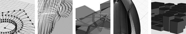
Fig. 1. Basic elements (Geometrical Complexity)
Basic elements category evaluates models according to the type of its most advanced geometry. Starting from the simplest geometry – points and ending with the most advanced – solids. In many cases outcome models, submitted by participants had various types of elements: points, lines, surfaces and solids. In some cases, all elements (including intermediary geometrical structures, such as centre points and surface edges) were kept visible, in other cases only resulting geometry was left visible. That is why the score was not awarded to all the types of elements of the model, but only to the most advanced type of element geometry. Six types of basic elements geometry were identified (from simple to complex): ‘Points’ (a point can be defined by XYZ coordinates), ‘Lines’ (a straight line; can be defined by two points), ‘Curves’ (a curved or straight line, can be defined by two, three or more points [includes all splines such as polylines, curves, interpolated curves; and primitives such as: circle, ellipse, rectangle and polygon]), ‘Planes’ (a flat, two-dimensional surface), ‘Surfaces’ (a curved, three-dimensional surface) and ‘Solids’ (a solid three-dimensional geometric figure [includes closed surfaces]).
3.2 Composition Space (Dimensional complexity)
2D – [0] / 3D – [1]
While basic elements geometry can be two or three dimensional the distribution (composition space) of those elements can also vary. Two types of spatial compositions were identified: 2D Composition – a flat, two-dimensional distribution of elements and 3D Composition – a three-dimensional distribution of elements. In this category, more dimensions mean more complexity, that is why 2D compositions were awarded [0] points and 3D compositions were awarded [1] point.
3.3 Arithmetic of Shapes (Shape Grammars)
Addition – [0] / Subtraction – [1] / Cull Pattern (Reduce or add elements according to a certain logic) – [2]
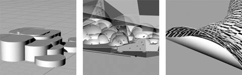
Fig. 2. Arithmetic of Shapes (Shape Grammars)
Arithmetic of Shapes is a category concerning operations which can happen when geometrical shapes intersect. They are often referred to as Boolean Operations or when elements have been culled according to some mathematical function or condition. ‘Addition’ (+) is an operation of transformation of two or more intersecting objects into a single object, such as the union of Region, Mesh or Solid. ‘Subtraction’ (-) is an operation that is opposite to 'Addition' and occurs when intersecting objects are being deducted from one another (such as Curve, Surface or Solid Trim and Region, Mesh or Solid Difference). ‘Cull Pattern’ is an operation of selecting certain elements and deleting or transforming them, such as Cull Index, Cull Pattern (true/false), Random Reduction etc. As the Evaluation method of model complexity is based on visual analysis of 3D models, it is often difficult or next to impossible to define if an ‘Addition’ operation has been performed. In many cases, when several shapes or volumes intersect they form a complex geometry and it is difficult to tell if they have been transformed into a unit or if they are separate and just intersect. That is why, in order to avoid confusion, ‘Addition’ operations were given [0] points. ‘Subtraction’ operations were given [1] point and ‘Cull Pattern’, as a more complex function, was given [2] points.
3.4 Transformations (Shape Grammars)
Scale – [1] / Rotation– [1] / Reflection – [1] / Deformation – [1] / Translation – [1]
The Transformation category is closely related to the ‘Arithmetic of Shapes' category, as it also deals with operations, which geometric elements of the 3D model undergo. Transformations are divided into five clearly identified types: Scale, Rotation, Reflection, Deformation and Translation. Each type of transformation is given one point. In many cases a combination of transformations takes place, where elements of the model are both rotated and scaled for example. ‘Scale’ is a type of transformation which deals with the elements size change. ‘Rotation’ is the process of turning the element around a centre or an axis. ‘Reflection’ is a type of transformation in which one element is the mirror image of the other. ‘Deformation’ includes a variety of operations dealing with shape changes, such as Bend, Twist, Blend and Morph. ‘Translation’ is the process of moving an object from one location to another. In practice, when looking at the resulting 3D model, it is near impossible to tell for certain if objects (model elements) have been moved (as a copy) or if the same objects have been generated in different locations. That is why, to avoid all uncertainties regarding the type of underlying modelling logic, in the cases where the same elements (same type of elements) has reoccurred in different locations it has been considered to be a ‘Translation’. According to pilot study results, ‘Translation’ is the most frequently used type of transformation. Only five models from fifty were developed without ‘Translation’ and in all those cases ‘Rotation’ transformation had been used.
3.5 Number of Elements (Components)
One Element – [0] / Two-Ten Elements –[1] / Multiple Elements (one Type) –[2] / Multiple Elements (’N’ Types) –[1 +’N’]
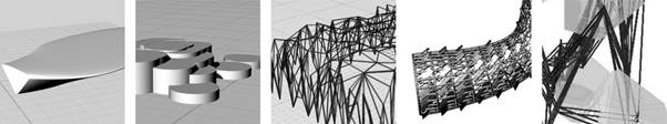
Fig. 3. Number of Elements (Components)
The ‘Number of Elements’ category is more obvious. It categorises models into four types of groups. The first group, ‘One Element’ is considered to be the most simple – [0] points. The second group of models are those that have from two to ten (same type) elements (nine cylinders for example) – [1] point. The Third group is ‘Multiple Elements’ have more than ten; they have the same type (for example a structure composed of hundreds of pipes) – [2] points. The last group in this category ‘Multiple elements (‘N’ Types), where ‘N’ stands for a number of types of elements (for example, when a model contains planes, surfaces and different types of solids). The score for this group is calculated according to the following expression: [X= N +1] points, where N stands for a number of types of elements.
3.6 Shape of the Element
Standards and Primitives – [0] / Non-standard Simple Shape – [1] / Complex Shape – [2]
The ‘Shape of the Element’ category evaluates the nature of element form making. When ‘Standards and Primitives’ (such as a circle, cube, sphere etc.) are used [0] points. In cases when a certain type of elements has a repeating ‘Non-standard Shape’ (like rhombus shaped surfaces with filleted corners) [1] Point. The third group includes elements, which have a non-repeating nature, meaning they are modified same-type elements (for example, extruded sections of a bubble shaped volume). These are referred as ‘Complex Shape’ elements and are given [2] points.
3.7 Colour
No colour – [0] / OneColour – [1] / Multiple Colours – [2] / Colour Gradient – [3]
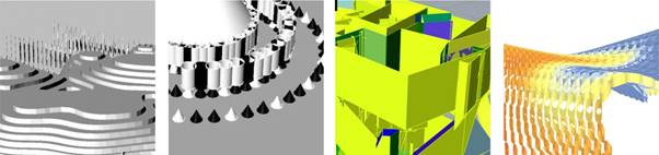
Fig. 4. Colour
The final category deals with the use of colours (shades) in the model. First group of models is models with ‘No colour’ – [0] points. When at least ‘One colour’ is used the model gets [1] point. Models, which elements or surfaces have ‘Multiple Colours’ get [2] points. When complex shading materials or ‘Colour Gradients’ are used, it is [3] points.
4.0 Experimental results
The total score for models submitted during the first and second workshop days varied from 4 to 33 points. It should be noted that only one person had developed more than one model. That is why the total score for this submission was much higher: 30 points (on day one), 33 (on day two) compared to the next best score of 16 points (day one) and 17 points (day two). All models were categorised into five different groups, the range was calculated as following: First Group (Most Simple Models): 0-6 points; Second Group: 7-9 points, Third Group: 10-12 points; Fourth Group: 13-15 points, Fifth Group: 16-33 points (See Fig. 5). The average score for the second assignment was approximately four points higher compared to the first assignment, but the overall complexity distribution curve had very similar (almost identical) shape. The clear majority of models were within the 10-12 and 13-15 point’s classifications.
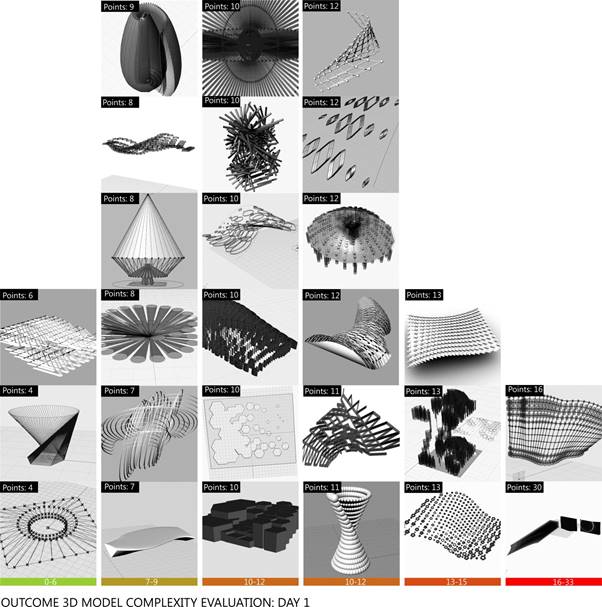
Fig. 5. Outcome Model Complexity Evaluation: Day 1
Prior to calculating the scores following the logic of the Model Complexity Point System, all models were sorted into five groups from simple to most complex, according to simple visual comparison (personal judgement). It should be noted that the majority of models in both types of analysis matched the complexity group choice. Visually simple models – were given fewer points and visually complex models were given higher scores. Although, a fair number of models were within the middle of the spectrum of complexity (according to the Point System) they appeared to be more complex than anticipated. Some models scored more points than expected and were sorted into groups with higher complexity.
These Metrics were successfully implemented as a practical method to evaluate the complexity of 3D models developed by Parametric Modeling Workshop participants using Grasshopper for Rhino. In theory, these Metrics are applicable for any geometric models including, virtual and physical.
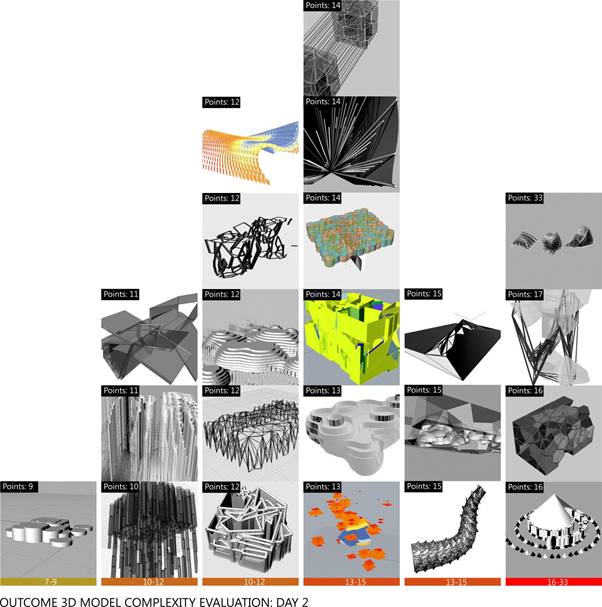
Fig. 6. Outcome Model Complexity Evaluation: Day 2
5.0 Discussion
The choice of characteristics system caused by the tasks that were set before the participants of the experiment to build and render the shape on a private example with a time restriction. Therefore, one of the key characteristics for building the model was the speed of building the model, measured in astronomical time. In this regard, the number of generated elements of the model was limited. Building a shape of 3D models based on a previously known representation of classification the three types of 3D models based on the measurement of the shapes complexity (by Forrest) with classification for linear planar and curved geometry.
Then a ballroom method of results evaluation of obtained 3D shape in the course of the job is used and complexity of 3D models is determined by the number of points. Seven categories are determined in accordance with different model groups, in turn, groups of models depend on a combination of three types of shapes geometry (according to Forrest).
A basic characteristic is the dimensionality of space, which is the rendered shape. In this design task, it is advisable to use 2 types of spatial dimensions: 2-dimensional and 3-dimensional.
The following basic characteristic – "The grammar of shape" that identifies the result or consequences of the interaction (intersection) of different geometry shapes. This characteristic suggests a three way interaction that determines the geometry complexity.
Next we introduce the characteristic that required building the shape – "The Transformation of shape" or the four most known transformation methods. These methods are equivalent in their complexity, but have different effects on shapes geometry; therefore, each selected method is evaluated equally. Perhaps, it would be to modify this section of the study, because it is not spelled combinations of different ways of transformation the same shape, but it may be the subject of further experiment in the field of transformation and grammar shapes. So we were limited to using only one transformation method to construct a single geometric shape.
The experiment results with quantitative assessment of simulation development the shapes of various complexity, determines the classification of models according by the complexity degree of the build. The index of difficulty expresses the summed scores on the various obtained variants: from minimum number in the range from 0 to 6 – "The Most Simple", to the maximum number from 16 to 33 points – "The Most Difficult", and intermediate evaluation options of complexity degree. For the tasks in this study was enough to determine the group of complexity. Therefore, we used the arithmetic method of identifying groups of 3D models, that collected approximately equal the number of points that were sorted by groups. These groups were sorted by two indicators: the number of points from 0 to 33 and the number of assignments that scored some points for relevant characteristics. Thus, on the basis of a two-day total result, we identify five basic degrees of models complexity: "The Most Simple", "Simple", "Medium", "Difficult", "The Most Difficult".
On the basis of obtained results, we can rely on the proposed methodology for complexity evaluating of the geometrical shape with compliance of all experiment conditions and given the defined characteristics of build the geometrical shape.
References
1. Cui J., Tang M.X. Integrating shape grammars into a generative system for Zhuang ethnic embroidery design exploration. Computer-Aided Design, Volume 45, Issue 3, Pages 591–604, Elsevier, March 2013
2. Forrest A. R. Computational geometry. Achievements and problems. Computer aided geometric design, Academic Press 1974.
3. Garland M. Quadric-based Polygonal Surface Simplification. PhD thesis, Carnegie Mellon, University, 1998.
4. “Grasshopper 3D” 2013. URL: http://www.grasshopper3d.com/ (accessed 23 July 2013).
5. Heisserman J. Generative geometric design. IEEE Computer Graphics and Applications, 14 (1994), pp. 37–45
6. Michael Garland. Quadric-Based Polygonal Surface Simplification. PhD thesis, Carnegie Mellon University, CS Dept., 1999.
7. “Rhino3d“: 2012. URL: http://www.rhino3d.com/ (accessed 23 July 2012).
8. Shah J.J., Smith S.M., Vargas-Hernandez N. Metrics for Measuring Ideation Effectiveness, Design Studies, 24:2, 111-134
9. Shikhare D. Complexity of Geometric Models, National Centre for Software Technology, Mumbai, 2001.
МЕТРИКА ИЗМЕРЕНИЯ УРОВНЕЙ СЛОЖНОСТИ ГЕОМЕТРИЧЕСКИХ МОДЕЛЕЙ
А.А. Глоба1, М. Донн2, О.А. Ульчицкий3
1Университета Дикина, г. Мельбурн, Австралия;
2Университет Виктории, г. Веллингтон, Новая Зеландия;
3ФГБОУ ВО «Магнитогорский государственный технический университет им. Г.И. Носова», г. Магнитогорск, Россия.
globalnaya@gmail.com, michael.donn@vuw.ac.nz, o.ulchitsky@magtu.ru
Аннотация
Данное исследование рассматривает практическую методологию для измерения уровня сложности геометрических моделей в архитектуре. Критерии для формирования метрики сложности моделей включают в себя геометрические, комбинаторные и пространственные категории. В исследовании также использована методология «Грамматика формы» (Грамматика поверхности), основанная на графических расчётах и логическом анализе формообразующих механизмов. В данной статье рассматривается теория и методология измерения геометрической сложности моделей и иллюстрируется практическое применение этого анализа на пятидесяти параметрически генерируемых 3D-моделей.
Исследование было проведено в рамках более широких исследований, оно фокусировано на параметрическом моделировании и способах поддержки использования параметрического проектирования за счет уменьшения объема программирования, а также увеличения рассматриваемых пространственных решений, программирования эффективности, степень проработки алгоритмозаписи и скорость алгоритмического моделирования (уровень сложности модели). Исследование включает ряд семинаров по параметрическому моделированию. Для того чтобы обеспечить экспериментальные данные для этого исследования, участники разработали и представили практические задания и заполнили онлайн-анкеты. Эта статья объясняет «шаг за шагом» методики определения сложности геометрических моделей и иллюстрирует практическое применение этого анализа для результатов моделирования, по результатам первого семинара.
Ключевые слова: сложность модели, архитектурная модель, параметрическое моделирование, грамматика форм, компьютерное проектирование, анализ геометрической модели.