SOLUTION OF PROBLEMS IN MODELING AND VISUALIZATION OF PROCESSES IN THE MICROWAVE DISCHARGE PLASMA
Yu.A. Lebedev, A.V. Tatarinov, I.L. Epstein, V.N. Timakin*, I.A. Tkachenko*
A.V.Topchiev Institute of Petrochemical Synthesis of the Russian Academy of Sciences
* National Research Centre “Kurchatov Institute”
lebedev@ips.ac.ru, atat@ips.ac.ru, epstein@ips.ac.ru, vtim@kiae.ru, tia@grid.kiae.ru
Contents
2. Creation of the specialized environment for computation and visualization
2.1. Architecture of the computation and visualization
2.2. Usage of the built environment to solve the problems
2.3. Access and security policies
3. Description of the used model and conditions of the simulation
4. Parameters of the simulation procedure and visualization
Abstract
In the article the relevance of development of specialized hardware-software complexes for visualization, the enhancement of algorithms of visual representation of data and the extension of opportunities of data display systems are discussed. Creation of a specialized distributed environment in order to solve 3D interactive visualization tasks of numerical simulation results of microwave discharge is described. Visualization of a computing mesh allowed to make visual estimates and to introduce necessary amendments in interactive mode. The realized distributed architecture of visualization supports easy migration of computing environment between instrumental visualization tools (consolidated or client's), providing an opportunity to scale the total amount of data and resolution of the images. Results of 3D visualization of the spatial distribution of the microwave field strength are shown on the example of a self-consistent simulation of argon plasma generated by means of the Beenakker cavity. The Spatial visualization by means of local cross sections of the computational domain let us discover an internal structure and features of the distribution of electron concentration in the discharge tube.
Keywords: simulation of the low-temperature plasma, data analysis, scientific visualization, scientific research, application software, visualization of data.
1. Introduction
Modern experimental methods of diagnostics and fast development of information technologies allow collecting and processing of very large volumes of information (Tera- and Petabytes) during a research of difficult objects, including the distributed computations. In recent years the exponential growth of data generation is being observed which exceeds our abilities to use it for scientific purposes and to control correctness of the received results in real time.
In order to understand simulation results of large data volumes, new approaches to the analysis and visualization and also creation of workflow management systems to perform storage and processing of big data in the distributed heterogeneous computer environment are required [1, 2].
All this confirms relevance of development of specialized hardware-software complexes for visualization, enhancement of algorithms of visual data representation, extension of opportunities of data display systems, including, stereoscopic and systems of ultrahigh resolution (tens and hundreds megapixels).
Data handling systems under such conditions have to comply with special requirements:
• the result of data handling under such conditions should be visual images which are easier perceived by the human brain and allow to understand the whole picture;
• scientific data processing and visualization should be connected into a general process allowing to obtain on the output a product which is convenient for a visual assessment of the received results in interactive mode;
• the data handling system should centralize and consolidate high-performance computing and visualization resources, with a possibility of remote and safe access.
The system of visualization of images can be both a dedicated software product and a component of an integrated hardware-software solution in a stack of a specialized data handling package. The structure of the visualization package and requirements imposed on it (for example, possibility to execute on different operating systems, on different hardware platforms; specific license requirements), define, eventually, the architecture of the whole hardware-software complex.
Technologies of visualization are most often applied in tasks of numerical modeling of complicated, multicomponent models when teraflops computer performance is required [2, 3].
Because of high complexity of the researched objects combined mesh creation can present considerable difficulties during the computation. The choice of the mesh sizes and structure, required for the solution of the specified problems with acceptable accuracy, implies changes in model parameters while analyzing the results of visualization and adjusting the mesh settings. Thus, the process of solving the problem of initial data analysis by the method of scientific visualization becomes more complicated: iterative and interactive [1, 4]. That is, in order to obtain results it is necessary to execute an algorithm of calculation and visualization repeatedly, all or its part, changing values of the parameters and carrying out a visual assessment of the intermediate results in real time.
Visualization of simulation results is gaining a special role in low-temperature plasma research. At the present time existent self-consistent models include a system of equations that describes plasma electrodynamics (dc discharge, LF, HF, UHF and optical discharges), kinetic processes (ionization, excitation, transport of charged and neutral particles, chemical reactions, phase transitions, the interaction of plasma with solids, and so on.), plasma gas dynamics, and heat transfer [5-8].
In recent years, there has been a rapid growth of works devoted to self-consistent modeling of complex systems in gas-discharge plasma [9-10]. It is explained by two reasons. Firstly, this is accumulation of reliable databases with various constants used in simulation (cross sections of different processes and reactions, transfer coefficients, and so on). Secondly, the increase of computer power allows to complicate formulation of problems, to bring the simulations closer to the description of the experiments and, moreover, to obtain results in reasonable time.
Moreover, if previously the zero-dimensional, one-dimensional and two-dimensional (2D) problems were solved, the advent of powerful computing resources makes it possible to develop three-dimensional models.
Creation of a distributed computing environment for interactive visualization of results of the numerical modeling of the argon plasma generated by the Binakker's microwave discharge was the purpose of the paper.
To achieve the goal, it was necessary to make the following steps.
A. To create a distributed specialized environment which should ensure:
• carrying out computation and post-processing on high-performance resources of a cluster complex;
• user access to the computing nodes to control the computational parameters, its launch and optimization of the resources;
• provision of a graphic console for remote interactive visualization of simulation results;
• protected remote access to the cluster resources;
• consolidated resources for remote rendering;
• mapping of high resolution data.
B. To simulate argon plasma of microwave discharge generated by means of the Beenakker cavity.
C. To carry out the analysis of results by the iterative and interactive 3D method of visualization.
2. Creation of the specialized environment for computation and visualization
2.1. Architecture of the computation and visualization
In order to achieve efficient use of computing resources, their clustering is applied, that is combining many computing nodes in a network with a single entry point and with the internal architecture hidden from users, Fig. 1.
Since the computing environment should allow not only simulation, but also results visualization, including interactive mode, it was necessary to use different node types (a heterogeneous cluster) in composition of the computing environment.
Thus, the created computing environment based on a heterogeneous computing cluster included:
• Nodes for computation on CPU;
• Nodes for computation on GPU;
• Hybrid computing nodes allowing to carry out computation both on CPU and GPU;
• Visualization nodes (assigned to operate with images and animation) – as the consolidated visualization resources;
• High resolution display system (video wall);
• Service nodes;
• Remote graphic station (client part);
• Set of programs for the downlink and safe functioning of the environment, simulation and visualization.
Slurm was chosen as a resource manager with a specially created set of scripts for preliminary processing of the launched jobs. It allows the user, unlike standard decisions, to be connected directly to a node where the computing and visualization task is launched, to see the result and, if necessary, to adjust or vary model parameters in interactive mode.
Since all nodes should have the same user data, a file system of network access - NFS with a source on a head node where users can copy the files for the subsequent calculations was set up.
The computing module of the application package has been integrated into the computing resources on the cluster. At the same time, modules of the control and postprocessing were installed either on remote resources of the user, or on nodes of the visualization cluster created as a consolidated resource. Thus, within the created environment two approaches to architecture of visualization were made.
In order to solve the interactive visualization problem, virtual displays were set up on the visualization cluster nodes. The virtual displays were not associated with real displays, the images were processed by means of the video card and results were interactively available to the remote client via the help of the graphic console.
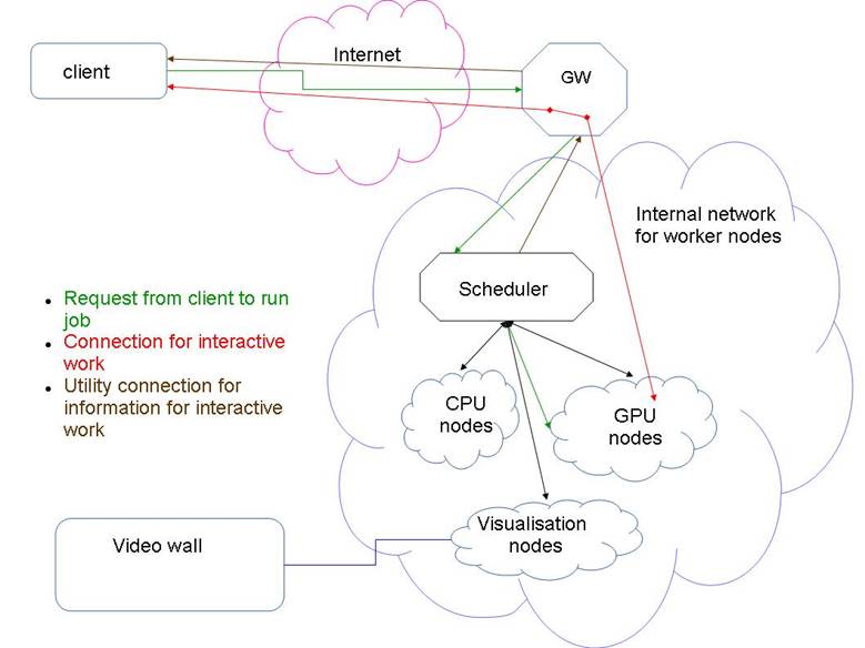
Fig. 1. Architecture of the computing environment.
In case of necessity of output of the visualization results in high-resolution, an opportunity to transfer a video content to a video wall in real time was developed. The Consolidated visualization tool consists of the following elements: cluster of visualization - optic line - video wall. The Video wall is located in a conference hall remotely from the cluster of visualization, the computing cluster and the data storage, which were integrated into a common environment by a high-speed data bus Infiniband. The video signal from the graphic visualization cluster cards was fed through optical lines on the video wall which consists of 12 thin-frame FullHD panels. The Total resolution of the video wall was 7680×3240 pixels. A structural feature was the use of a software solution to manage the wall. We used the SAGE software [11]. SAGE provides common environment enabling its users to access, display and share a variety of data-intensive information, in a variety of resolutions and formats, from multiple sources, on tiled display walls of arbitrary size.
The created specialized environment allows users to solve a wide range of problems, and, at the same time, gives them a possibility of an individual approach to every problem if it is required. For example, in order to launch a client part of application designed to operate in Windows, a possibility to launch virtual machines on the cluster of visualization under VirtualBo? control was implemented, with a possibility to access from the virtual machine to the GPU-card of the nodes. Thus, according to one approach rendering of results could be carried out on scalable resources of the visualization cluster.
An Other approach considered specifics of the used application package and provided a possibility to set up the visualization module on a user’s workstation. For this case the client-server architecture was implemented.
2.2. Usage of the built environment to solve the problems
The Comsol Multiphysics v. 3.5a package [12] was used as a computing device, (License № 1064223). This package is designed to conduct finite and element analysis in different areas of physics and engineering, including the coupled (multiphysics) problems. There are specialized modules in the package that are used for specific disciplines, and effective interaction between all modules is provided for solving the interdisciplinary problems.
It was impossible to use the packet directly to install it on the computing cluster. We divided it into two modules: a computing module and a client module (control and monitoring over the process of computing and visualization). An important condition for the computing module integration to our computational environment was its separation from the Comsol software package in order to install the module on the cluster nodes in the Linux operating environment. The Computing module was to be set in a HPC nodes and operate without use of the graphical interface. One computing node of HPC was used as hardware resources: SL390 (3 GPU nVidia Tesla M2050, 48Gb RAM, 2 Intel Xeon X5670). A choice of the node with graphic cards was made to study possibility of rendering in a remote cluster within this application software. The most effective solution, from the point of view of software and hardware tools, is to use the high-performance resources of HPC for both computation and postprocessing (visualization of the data).
The client part is responsible for managing calculation and postprocessing processes. In the implemented architecture it was installed on the remote client graphical station that runs on MS Windows operating system due to the client-side operating system requirements and the license agreement. As the result, the computing control and visualization of data were carried out on the remote graphic station which was accessible to HPC via public network infrastructure.
Since the computing module that was isolated from the application package did not allow interactive installation without using the graphical interface, we created a special script at this stage to carry out the procedure of installation in automatic mode. In order to use graphic cards resources during the start of the computing module, we created a virtual display using an X server which had no connection to any physical output device of the image. We did not succeed in the complete exclusion of the graphic cards from the computing module operation.
In case if optimization of the computations was needed the user could vary the number of cores in computing nodes at the startup of the computation.
2.3. Access and security policies
The Remote access to the computational resources should be carried out as safe as possible for the user and the resource center. Insufficient attention to the security policy can lead to the fact that computing resources will be in the hands of criminals who can use them, for example, to hack other secure systems. Also the whole software should be checked for vulnerabilities. The computing module (CM, see below 2.3) of the used applications is not safe enough for using it through the public Internet. Accordingly, CM was protected by firewall allowing remote access only from specific IPs.
Since the end-user has no static IP address, an additional transit server was configured allowing the SSH access from the selected IP. Further, by means of SSH tunneling through a transit server the secure, encrypted channel between the user and the computing module is created. Moreover, to avoid potential problems with HPC (high performance cluster) side in case when the client is hacked, the transit server was specially configured to start automatically or stop CM at the HPC-nodes when the client connects or disconnects. It was made in the automatic mode by means of commands and batch scripts, not allowing the user to take any action at both the transit and the HPC-node.
3. Description of the used model and conditions of the simulation
We used a self-consistent 3D model of the non-equilibrium non-uniform microwave discharge in a nonlocal approximation. The model is based on the simultaneous solution of Maxwell’s equations, Poisson equations, Boltzmann's equations for the free electrons of plasma and the equations that describe oscillatory kinetics and kinetics of excited and charged particles of plasma. Computing algorithms are discussed in the articles [5-8] in more details. In order to describe plasma, a drift-diffusion approximation for the steady-state flows of particles is used, [29, 30]. Balance equations for electrons, ions (Ar+ and Ar2+) and Ar atoms in the electronically excited states are written in the following form:
|
|
|
|
|
|
|
(1) |
|
|
|
(2) |
|
|
|
(3) |
Here Γe , Γip , Γin, ne , nip , nin are flows and density of electrons (e), ions (p) and neutral particles (n) of the i-th type; Sie,p,n is the total production and loss rate of relevant particles of the i-th type in various plasma-chemical processes; μie,p , Die,p,n are coefficients of the mobility and diffusion of relevant particles of the i-th type, and Ec = -Ñj is a local electric field due to the charge separation, calculated from the Poisson equation for the potential φ:
|
|
(4) |
where e is the electron charge, ε0 is the permittivity of vacuum.
Since in studied conditions and geometry of the discharge system the relaxation length of electron energy significantly exceeds the radius of the discharge tube a self-consistent model in a nonlocal approximation is used for the description of the discharge [28].
In this case the local connection of the parameters of the electronic component with microwave field is absent; it is replaced by the balance equation of the electron energy density [29, 30]:
|
|
|
(5) |
where Γε is the flux of electron energy density with coefficients με = 5/3 μe, Dε = 5/3 De , ε is the electron energy density associated with mean electron energy θ as ε = ne·θ, θ = 3/2 kB·Te, kB is the Boltzmann constant, Te is the electron temperature. The Qin term identifies energy losses of electrons in the inelastic collisions; Qel identifies energy losses of electrons in the elastic collisions; σ is the plasma conductivity.
The electric component of the microwave field Em is calculated from the dynamic Maxwell equations. In the case of stationary structure of TM waves established in the resonator, the Maxwell equations are reduced to a singular complex equation for a magnetic component of the wave:
|
|
(6) |
Here ![]() is the relative permeability and conductivity
of plasma, where the electron density ne is normalized to its
critical value nc ≈ 7×1010 cm-3
for a given microwave frequency f = 2.45 GHz. The relative magnetic
permeability of the plasma μr is equal to one, νcol
is a collision frequency of electrons with neutrals.
is the relative permeability and conductivity
of plasma, where the electron density ne is normalized to its
critical value nc ≈ 7×1010 cm-3
for a given microwave frequency f = 2.45 GHz. The relative magnetic
permeability of the plasma μr is equal to one, νcol
is a collision frequency of electrons with neutrals.
The model contains pre-computed table files with the rate constants of reactions which include an electron impact. These rate constants are functions of the local values of the mean electron energy θ and electron concentration ne. The electron energy distribution functions, needed for the calculation of those constants, have been obtained by solving the Boltzmann equation for the free electrons of the plasma in the two-term approximation with a self-consistent set of cross sections for argon.
In order to achieve a correct simulation, we need to account on a large number of electronic excited states of atoms and molecules, oscillatory distribution of molecules, several types of ions.
Table 1 shows the processes included in the kinetic model. The following electronically excited states of argon atoms have been taken into account:
- 4 lower electronic states are combined into two states: metastable state Ar(M) ≡ (1s5)+ Ar(1s3) and resonant state Ar(R) ≡ Ar(1s2) + Ar(1s4).
- to simplify the kinetic scheme by analogy with [27, 28] the states with high energy excitation threshold are combined into three lumped levels Ar(F, A and B): with level Ar(F) (13.2 eV) being the sum of the 3p54p levels, level Ar(A) (14.1 eV) being the sum of the 3p55s and 3p53d levels and level Ar(B) (14.9 eV) being the sum of the 3p56s, 3p55p, 3p54d and 3p54f levels.
Table 1. Processes in the argon plasma incorporated in the model.
|
No. |
Process |
k(?m3s-1, ?m6s-1); Ai (s-1); |
References |
|
Excitation from the ground state |
|||
|
1 |
Ar + e → Ar(M) + e |
f(θ,ne) |
[13] |
|
2 |
Ar + e → Ar(R) + e |
f(θ,ne) |
[13] |
|
3 |
Ar + e → Ar(F) + e |
f(θ,ne) |
[13] |
|
4 |
Ar + e → Ar(A) + e |
f(θ,ne) |
[13] |
|
5 |
Ar + e → Ar(B) + e |
f(θ,ne) |
[13] |
|
Stepwise excitation |
|||
|
6 |
Ar(M) + e → Ar(F) + e |
f(θ,ne) |
[14, 15] |
|
7 |
Ar(R) + e → Ar(F) + e |
f(θ,ne) |
[16] |
|
8 |
Ar(F) + e → Ar(A) + e |
f(θ,ne) |
[17] |
|
9 |
Ar(F) + e → Ar(B) + e |
f(θ,ne) |
[17] |
|
10 |
Ar(A) + e → Ar(B) + e |
f(θ,ne) |
[17] |
|
Direct, stepwise and chemi- ionization |
|||
|
11 |
Ar + e → Ar+ + e + e |
f(θ,ne) |
[18] |
|
12 |
Ar(M) + e → Ar+ + e + e |
f(θ,ne) |
[19, 20] |
|
13 |
Ar(R) + e → Ar+ + e + e |
f(θ,ne) |
[19, 20] |
|
14 |
Ar(M) + Ar(M) → Ar+ + Ar + e |
α×1.2×10⁻⁹ |
[21] |
|
15 |
Ar(M) + Ar(M) → Ar2+ + e |
(1-α)×1.2×10⁻⁹ |
[21] |
|
16 |
Ar(M) + Ar(R) → Ar+ + Ar + e |
α×2.1×10⁻⁹ |
[21] |
|
17 |
Ar(M) + Ar(R) → Ar2+ + e |
(1-α)×2.1×10⁻⁹ |
[21] |
|
Mixing by electrons |
|||
|
18 |
Ar(M) + e → Ar(R) + e |
2.35×10⁻⁷ |
[21, 22] |
|
19 |
Ar(R) + e → Ar(M) + e |
3.1×10⁻⁷ |
[21, 22] |
|
Dissociative recombination |
|||
|
20 |
Ar2+ + e → Ar + Ar |
1.1×10⁻⁷×Te-0.5 |
[27] |
|
Emission |
|||
|
21 |
Ar(R) → Ar + hν |
teff -1 = 1.19×10⁸ × gesc |
[23-25], see the text |
|
22 |
Ar(F) → Ar(M, R) + hν |
teff -1 = tnat -1× gesc |
[23-25], see the text |
|
23 |
Ar(A) → Ar(F) + hν |
1.56×10⁷ |
[28] |
|
24 |
Ar(B) → Ar(A) + hν |
8.6×10⁶ |
[28] |
|
25 |
Ar(B) → Ar(F) + hν |
9.1×10⁵ |
[28] |
4. Parameters of the simulation procedure and visualization
Geometry of the model. The system geometry and sizes of the resonator, used in simulations, are given in Fig. 2. An argon discharge is ignited inside the quartz tube 18 cm in length with its inner 5.2 mm and outer 6.8 mm diameters. The gas pressure inside the tube is set to 0.5 Torr. Height of the cylindrical part of the resonator (3) - 7.7 mm. The quartz tube passes through the resonator’s axis of symmetry. The quartz tube is surrounded by a virtual cylinder of a larger diameter outside the upper and lower metallic plates of the resonator. The external parts of the tube outside the resonator are equal in length. The vertical coaxial wave guide (1) is part of the microwave feeder. At the top plane of the coaxial segment with the rod antenna an ideal non-reflective source of TEM wave with λ0 = 12.45 cm is specified. The tuning quartz rod (5) goes through a narrow cylindrical wall of the cavity, it is being moved inside until the plasma column ignites. The resonator is excited by a coaxial feeder with an inner rod antenna (2), vertically entered through the top cover of the cavity. Its end face was in the middle between the upper and lower plates of the resonant cavity.
Boundary conditions and the simulation procedure. System of equations (1)-(6) is augmented with the geometry of the model and the following boundary conditions. The normal component of the magnetic field was assumed to be zero at infinitely thin metal surfaces of the resonator. Since the gas flow realized in experiments has no influence on the kinetic processes in plasma, both ends of the discharge quartz tube are assumed sealed in simulations.
On the walls of the cylinders a scattering condition without reflection is set for any incident wave. At the top plane of the coaxial segment with the rod antenna an ideal non-reflective source of a TEM wave with λ0 = 12.45 cm was placed.
It is known that in resonators with low Q-factor the electron density of the microwave plasma is above the critical value nc [26]. We also know that in the argon plasma at such pressures characteristic value of the average energy is 3-5 eV. The characteristic energy density for such a discharge is εc ~ 3-5×10¹¹ eV·cm-3. We expect that near the inner boundary of the quartz tube the values of the electron density and energy density should be much smaller than the values nc and εc in the plasma volume. Preliminary simulations have shown that for any wall values which satisfy new < 0.01nc, εw < 0.02εc, the correspondent solutions are almost identical. Therefore, all further calculations were performed with the following boundary values for the electron density and electron energy density: new ≈ 5×108 cm-3, εw ≈ 5×10⁹ eV·cm-3. The density of Ar+ ion is set equal to new, concentrations of Ar2+ ions and of all excited argon atoms were set to zero on the walls.
Used visualization modules. We used a set of visualization tools from the Comsol Multiphysics system. Features of the package usage consisted in the fact that the control module (including visualization module) and computing module was divided, and the visualization module could be installed either on a remote workstation or on a cluster of visualization with data mapping on a video wall. At the same time, a full-featured remote access using the graphical user console for interactive visualization of the results was provided, due to addition of virtual displays during the installation of the computing module. When we used the visualization module of the Comsol system the following tools were applied: “Cross-Section Plot Parameters”, for the purpose of investigation of the parameters of the variables in the form of cross-sections of a 3D object; "Domain Plot Parameters" for the purpose of investigation of the variables on the boundary of the objects partition area. Arrow Plot mode was used for visualization of the vector of the microwave field. Slice mode was used to display the values of the parameters by the color in the selected plane.
We decided not to use the classical scheme of creating a video wall using the hardware controller and used the module of visualization from SAGE software package for managing video wall instead. We used the updated version SAGE2 [11], entirely rewritten on JavaScript platform. This enabled the transformation of data in order to display it on the wall in a "raw" form in real time directly from performing calculations programs. In addition, the package allows transferring the metadata to the remote visualization nodes running SAGE without any additional changes via network in real time, i.e. perform remote rendering of high resolution data. The important factor is that it is a free software package.
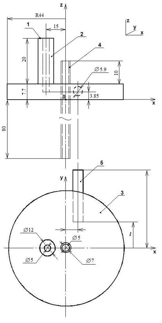
Fig. 2. Geometrical model parameters.
5. Results and discussion
The method of iterative and interactive visualization significantly simplified and accelerated simulation process. For example, the problems on convergence associated with non-locality of the problem were solved during the simulation. For understanding such parameters as convergence, a part of the tube limited by the resonator’s planes was selected for the first iteration of the simulation. That is, an area with the strongest electric field gradients was selected.
Fig. 3 shows calculations for an empty resonator and a part of the plasma tube.
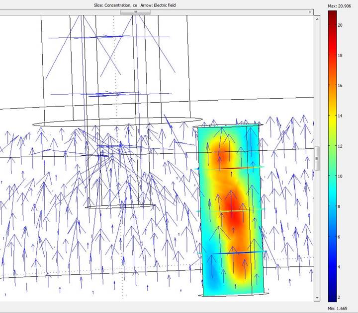
Fig. 3. Electron density and vectors of the electric field strength inside the resonator.
Here arrows show the electric field strength, and the colors reflect change of electron concentration in the tube. After a visual estimate of the received results and comparison of its similarity to the experimental data, the decision on transition to a model with real geometry was made. The simulation of a discharge with a real geometry requires a considerable number of mesh points. The choice of mesh point numbers is defined by the optimal ratio of the time spent on the calculations to the accuracy required for description of the studied processes. Since personal computers were used in the laboratory there was not enough random access memory (4 GB only), so the maximum number of degrees of freedom reached only 40000. The number of mesh points didn't exceed 6000. The computations were constantly stopping due to shortage of the resources.
The facilities of the created environment allowed us to continue simulation and to increase the number of mesh points. One of the variants of The first iterations of mesh points selection is shown in fig. 4. Visualization of a mesh allows estimating how well the mesh meets the accuracy criteria for each area and, if necessary, making appropriate adjustments to the meshing. The quantity of mesh points was increased in areas where the greatest changes of the electric field intensity were found.
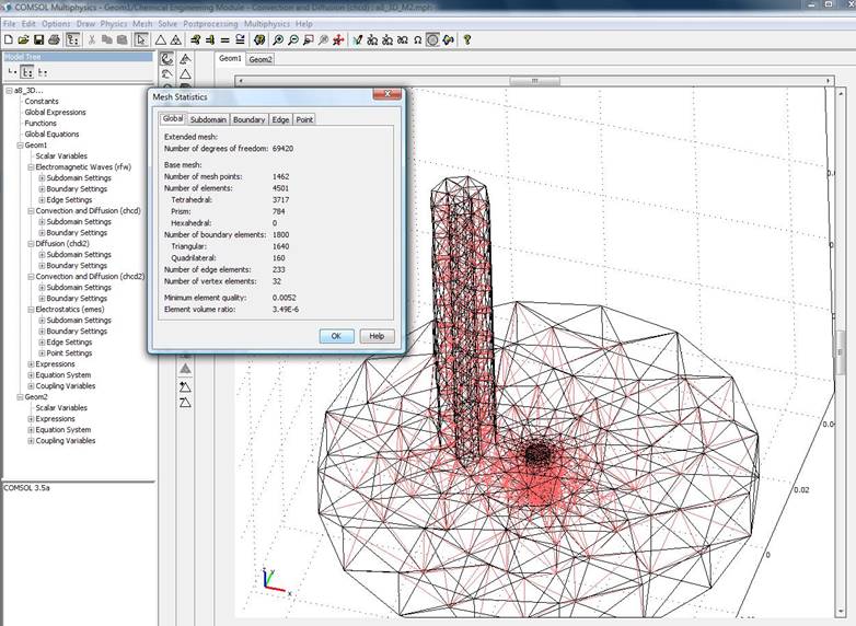
Fig. 4. Creation of a combined mesh in the computing area.
As a result of iterations, the convergence was observed. The following mesh settings were used to take into account all changes in the field strength (fig. 5): the number of degrees of freedom was more than 379 000, and the number of mesh points reached 7233. The Minimum linear cell size is 1 mm.
The Computation was carried out on a cluster node which consists of 12 CPU cores and 24 GB of random access memory. It was the CPU which worked the most actively during the computation process. Loading on the CPU cores was about 100% during the whole running time. The Memory usage was not more than 25%. The load on the cores of GPU accelerator was less than one percent, the use of GPU memory corresponds to the memory usage of a graphical environment. This means that the visualization module of Comsol package doesn't use GPU accelerators during the rendering of an image. According to the visualization process, we may assume that the current configuration and the way of its usage may be applied to ordinary computing nodes that have no special GPU cards if only these nodes are customized in the right way (with virtual displays support).
The first results of 3D visualization of simulation of the microwave discharge in argon are obtained for 3D problems for a system with a large number of degrees of freedom, using a simplified geometry of the microwave cavity.
Fig. 5. A combined mesh in the computing area.
Visualization of the spatial distribution of the electric microwave field is shown in fig. 6.
The Simulations showed that the plasma is divided into two areas: a central ellipsoidal core, mainly located inside the resonator and a little out of it, and a peripheral homogeneous column that uniformly fills the quartz tube outside the resonator. The microwave field is mostly concentrated inside the resonator with maximal values on the walls of the quartz tube. Outside the resonator the wave decays at a distance of a few millimeters.
In contrast to the microwave field the mean electron energy does not vanish at the exit of the resonator’s cavity, it remains constant and equal to about 3 eV.
Fig. 6. Vectors of the electric field strength in the empty resonator.
The possibility to use local sections inside the object of interest allowed to discover the internal structure and features of the computing parameters via three-dimensional visualization. The concentration of electrons in the discharge that was obtained from the computer simulation is shown in the following fig. 7. Here ce = ne/nc, ne is the electron concentration, nc = 7×1010cm-3 is the critical density of electrons, which corresponds to the frequency of the source wave.
Fig. 7. Electron density in discharge.
Launch of the Control and Visualization module of the applied packet allows to access a computational module by using a thin client (vnc) and relieves a user of the need to have a client side that is configured to work with the cluster, as well as increases the security of the cluster as a whole, since the client needs an access to a single node cluster by means of client-server solution with open source.
We used a visualization module of the software package SAGE, hence, we could make high-resolution data mapping from the cluster of visualization directly to a tiled display wall. It allowed us to do a more detailed visual assessment and a comparative analysis of the whole complex of the data at the same time, fig. 8.
Fig. 8. High-resolution data mapping from the cluster of visualization to a tiled display wall.
6. Conclusion
The distributed heterogeneous computing environment for simulating and 3D visualization has been created. It represents an integrated set of programs and controlling scripts which connect processes of storage with processing and visualization into a general system of computation with a uniform entry point.
Computation was executed by computer resources of Collective Usage Centre "Complex of simulation and data handling of research installations of a mega-class" at NRC "Kurchatov Institute".
The computing architecture that was Implemented in this environment enables:
- to analyze results of the simulation of the Beenakker's microwave discharge in argon by method of iterative and interactive visualization;
- to ensure a complete secure access for external users to computing resources and to provide a graphical console directly to computing nodes;
- to carry out a project creation in a single technological chain, monitoring and management of computational process and subsequent visualization of the data in an interactive mode, including the configuration with a remote access.
The realized distributed architecture of visualization supports an easy migration of a computing environment between the work benches of visualization (consolidated or client's), providing users with a possibility to scale the total amount of data and resolution of their images.
Results of the 3D visualization of microwave field strength have been obtained. The results showed that the field is mainly concentrated inside the resonator with the maximum values on walls of the quartz tube.
3D visualization in chosen cross sections of the computational domain allowed to discover an internal structure and features of the electron concentration inside the plasma tube.
References
[1] Pilyugin V., Malikova E., Pasko A., Adzhiev V. Scientific visualization as method of scientific data analysis. Scientific visualization. 2012. vol. 4. no. 4, pp. 56-70. [In Russian]
[2] Krinov P.S., Polyakov S.V., Iakobovski M.V. Visualisation in distributed computational systems of results of three dimensional computations. 4 International Conference of Mathematical Modeling: “Stankin”. 2001. v. 2, pp. 126–133
[3] Nesterov I.A. Interaktivnaja vizualizacija vektornyh polej na raspredelennyh vychislitel'nyh sistemah [Interactive visualization of time-varying flow fields using high performance parallel systems]. Matem. Mod. 2008. Vol. 20. no. 6, pp. 3–14 [In Russian]
[4] Bondarev A.E., Galaktionov V.A., and Chechetkin V.M. Analysis of the Development Concepts and Methods of Visual Data Representation in Computational Physics. Computational Mathematics and Mathematical Physics. 2011. vol. 51. no. 4. pp. 624–636.
[5] Jovovic J., Epstein I.L., Konjević N., Lebedev Yu.A., Šišović B., Tatarinov A.V. The Influence of Small Hydrogen Admixtures up to 5 % to a Low Pressure Nonuniform Microwave Discharge in Nitrogen. Plasma Chem. Plasma Process. 2012. 32. pp. 1093–1108.
[6] Lebedev Yu.A., Mavludov T.B., Epstein I.L., Chvyreva A.V., Tatarinov A.V. The effect of small additives of argon on the parameters of a non-uniform microwave discharge in nitrogen at reduced pressures. Plasma Sources Sci. Technol. 2012. 21. 015015.
[7] Lebedev Yu.A., Yusupova E.V. Vlijanie postojannogo polja na pripoverhnostnuju plazmu sil'no neodnorodnogo SVCh razrjada [Effect of the dc Field on the Near Surface Plasma of a Highly Nonuniform Microwave Discharge]. Plasma Phys. Rep., 2012, 38, No. 8, pp. 677–683. [In Russian]
[8] Shakhatov V.A., Lebedev Yu.A. Metod jemissionnoj spektroskopii v issledovanii vlijanija sostava smesi gelija s azotom na harakteristiki tlejushhego razrjada postojannogo toka i SVCh razrjada [Radiation Spectroscopy in the Study of the Influence of a Helium–Nitrogen Mixture Composition on Parameters of DC Glow Discharge and Microwave Discharge]. High Temp. 2012. Vol. 50. No. 5. pp. 663–686. [In Russian]
[9] Encyclopedia of Low Temperature Plasma, ed. V. E. Fortov, 2000, v. 1-4. Moskow: Nauka, [In Russian].
[10] Chemistry of Low Temperature Plasma, ed. Yu. A. Lebedev, N.A. Plate, V. E. Fortov. Moskow: Yanus-K, 2006, 480 p. [In Russian].
[11] SAGE2, http://www.sagecommons.org/.
[12] COMSOL 3.5a http://www.comsol.com
[13] Yanguas-Gil, Cortrino J., Alves L.L. An update of argon inelastic cross sections for plasma discharges. J. Phys. D. Appl. Phys. 2005. pp. 1588-1598
[14] Boffard J.B., Piech G.A., Gehrke M.F. et all. Measurement of electron-impact excitation cross sections out of metastable levels of argon and comparison with ground-state excitation. Phys. Rev. 1999. A 59. 2749
[15] Bartschat K., Zeman V. Electron-impact excitation from the (3p54s) metastable states of argon. Phys. Rev. 1999. A 59, R2552
[16] Gangwar R.K., Sharma L., Srivastava R., Stauffer A.D. Argon plasma modeling with detailed fine-structure cross sections. J. Appl. Phys. 2012. Vol. 111, Issue 5
[17] Drawin H.W., Emard F. Physica C85, 333, (1977)
[18] Rapp D., Englander-Golden P. Total Cross Sections for Ionization and Attachment in Gases by Electron Impact. I. Positive Ionization. J. Chem. Phys. 43, 1464,
[19] Hyman H.A. Electron-impact ionization cross sections for excited states of the rare gases (Ne, Ar, Kr, Xe), cadmium, and mercury. Phys. Rev. A. 1979. A20, 855.
[20] Dixon A.J., Harrison M.F., Smith A.C.H. in Abstracts of the VIII-th ISPEAC, Belgrad, 1973, p.405
[21] Karoulina E., Lebedev Yu. Computer simulation of microwave and DC plasmas: comparative characterisation of plasmas. J. Phys. D: Appl.Phys. 1992. Vol. 25. Pp. 401-412
[22] Ferreira C., Loureiro J., Ricard A. Populations in the metastable and the resonance levels of argon and stepwise ionization effects in a low‐pressure argon positive column. J. Appl. Phys. 1985. Vol. 57. Pp. 82-90
[23] H. van Tongeren. Positive column of the Cs–Ar low‐pressure discharge J. Appl. Phys. 1974. Vol. 45. 89
[24] Holstein T. Imprisonment of Resonance Radiation in Gases. Phys. Rev. 1947. vol. 72. Pp. 1212-1233
[25] Walsh P. Effect of Simultaneous Doppler and Collision Broadening and of Hyperfine Structure on the Imprisonment of Resonance Radiation. Phys. Rev. 1959. Vol. 116. Pp. 511-516
[26] Lebedev Yu.A., Polak L.S. High Energy Chem. HIECAP. 1980. Vol. 13. No. 5. pp. 331-348
[27] Biberman L.M., Vorob’ev V.S., Yakubov I.T. Kinetiks of Nonequilibrium Low-Temperature Plasmas. Moscow: Nauka, 1982; NY: Consultants Bureau, 1987.
[28] Dyatko N.A., Ionikh Y.Z., Kochetov I.V. et all. Experimental and theoretical study of the transition between diffuse and contracted forms of the glow discharge in argon. J. Phys. D: Appl.Phys. 2008. Vol. 41, 055204.
[29] Shkarofsky I.P., Johnston T.W., Bachynski M.P. The Particle Kinetics of Plasmas. Addison-Wesley PC. 1996.
[30] Hagelaar G.J.M., Pitchford L.C. Plasma Sources Sci. Technol. 2005. Vol. 14. Pp. 722-733.