A RESEARCH OF PROCEDURES USED IN THE ANALYTIC HIERARCHY PROCESS AND VISUALIZATION IN SENSITIVITY ANALYSIS
V.V. Kotova
National Research Nuclear University MEPhI (Moscow Engineering Physics Institute), Moscow, Russian Federation
e-mail: VNV.Kotova@gmail.com
Contents
3. Analysis of the AHP procedures
3.1. Comparison of eigenvector and geometric mean methods for deriving priorities
3.2. Analysis of consistency index
3.3. Analysis of linear aggregation
4.1. Tasks of sensitivity analysis and usage of visualization for solving them
4.3. Approaches to sensitivity analysis and visualization in them
Abstract
In this paper, the AHP, a multi-criteria decision method designed to solve hierarchically structured problems, is discussed. Two of its main procedures are reviewed in detail: pairwise comparisons that allow transformation of values measured on a physical scale into dimensionless numbers and derivation of weights and additive aggregation used to synthetize priorities. Drawbacks of the procedures are shown and substantiated, variants of their optimization and elimination are suggested.
In order to conduct sensitivity analysis, visualization methods are used. These methods permit the comparing of alternatives taking into account possible uncertainties, generate scenarios of possible rankings of decision alternatives under different conditions and assess the impact of changes of criteria weights on the result. In this case, the visualization serves as an argumentation base for the final decision, it allows to analyze a huge amount of tabular data within a limited amount of time.
Keywords: Analytic Hierarchy Process, Multi-criteria decision making, sensitivity analysis, visualization
1. Introduction
“The AHP is a comprehensive framework which is designed to cope with the intuitive, the rational, and the irrational when we make multiobjective, multicriterion and multiactor decisions with and without certainty for any number of alternatives”. This detailed definition of the AHP was given by Harker and Vargas in 1987 [1].
Structuring complexity, measurements on a ratio scale and synthesis of results are the three primary functions of the AHP. The method gives to an expert an opportunity to use all information he has, consider tangible and intangible factors. Moreover, the AHP provides an effective framework for group decision making, helps to rich a consensus and to evaluate competence of experts in case of their parallel work.
Sensitivity analysis is crucial to the validation and calibration of numerical models [2], obtained via the AHP. As the result of it, the expert obtains a large amount of tables. However, tabular data alone are not particularly helpful for the decision maker (DM) [3]. Thus, visualization have become widely used in data analysis tools in recent years [4]. Visualization helps to combine the strength of the human and computer [5]: creativeness and high-speed performance.
Many software applications provide different methods of graphical sensitivity analysis, including charts similar to charts in fig. 1. Visualization methods give an opportunity to compare alternatives under possible uncertainties, to evaluate robustness of the obtained result, to generate scenarios of possible rankings of the alternatives under different conditions and so forth.
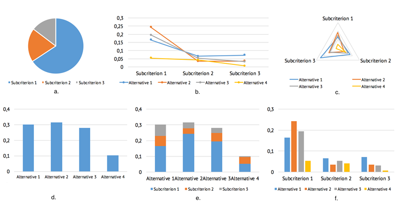
Fig. 1. Approaches to visual sensitivity analysis: a. criteria weights; b. parallel coordinate plot; c. partial ranking; d. alternatives ranking; e. aggregated ranking; f. alternatives comparison
GIS-based AHP gained high popularity because of its capacity to integrate a large amount of heterogeneous data and the ease in obtaining the weights of enormous alternatives (criteria), and therefore, it is applied in a wide variety of decision making problems [2]. In this case, input data values are directly plotted on the map. As an example, two pictures from [6] fig, 2 are represented below.
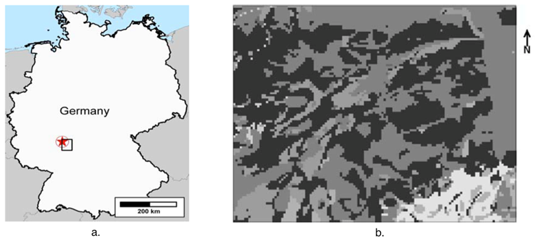
Fig. 2. Visualization methods in GIS a. map of Germany (the area of the research is outlined by the black square) b. expanded map of the area of the research
In this paper, the AHP is considered not only as a numerical method but as a framework, approach to solving decision making problems. In chapter 1 the principal procedures of the AHP are discussed. Chapter 2 is devoted to admissibility analysis of the procedures. The main objective of chapter 3 is to review sensitivity analysis and appliance of visualization methods on this stage of the AHP’s algorithm.
2. Review of the AHP
The AHP was developed by Saaty [7] and has gained huge popularity for solving applied problems in the last 30 years [8]. At the same time, many researchers have noticed its drawbacks [9,10]. One of them is the rank reversal phenomenon caused by alterations in the set of alternatives. The validity of some procedures is also a subject for ongoing debates.
However, many scientists support the AHP as described in the first publication [1]. One of the reason is that our world is inconsistent by its nature, hence, a method must not be applied only because it gives the results we want and expect to obtain [11]. Let us review the basic procedures of the AHP in more detail.
2.1. Problem statement
To begin with, we should define what type of problems can be
solved via the AHP and what type of an answer we will get as the result. The
problem should consist of a big amount of criteria ![]() using
which alternatives
using
which alternatives ![]() are
compared. Criteria that belong to the set
are
compared. Criteria that belong to the set ![]() form
a hierarchy defined by Saaty in [12].
form
a hierarchy defined by Saaty in [12].
A hierarchy ![]() is a
finite partially ordered set with the largest element
is a
finite partially ordered set with the largest element ![]() which satisfices the
following conditions
which satisfices the
following conditions
1. ![]() consists
of sets called levels
consists
of sets called levels ![]() where
where
![]() .
.
2. If ![]() is an element of the
is an element of the ![]() th level (
th level (![]() ),
then the set of elements “below”
),
then the set of elements “below” ![]() is a
subset of the
is a
subset of the ![]() st level
st level ![]() .
.
3. If ![]() is an element of the
is an element of the ![]() th level, then the set
of elements “above”
th level, then the set
of elements “above” ![]() is a
subset of the
is a
subset of the ![]() st level
st level ![]() .
.
As for four decision-making problematics firstly suggested
by Roy [13], the AHP addresses only two of them: the choice problematic ![]() and the ranking
problematic
and the ranking
problematic ![]() .
.
An example of a hierarchical problem structure is represented in fig. 3.
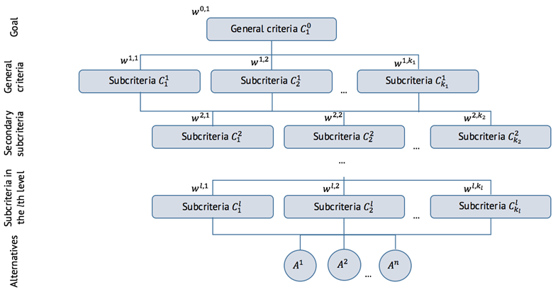
Fig. 3. Hierarchy
2.2. Algorithm
The generalized algorithm of the AHP is represented in fig.
4. At first, the analytic defines a set of alternatives ![]() and
criteria
and
criteria ![]() . In
the next step, the expert has to separate the criteria into several groups,
establish connections between these groups, build a hierarchy that complies
with the axiom 3 in [12]. The hierarchy must include the goal, primary and
alternative options to reach the goal, criteria to evaluate the alternatives.
. In
the next step, the expert has to separate the criteria into several groups,
establish connections between these groups, build a hierarchy that complies
with the axiom 3 in [12]. The hierarchy must include the goal, primary and
alternative options to reach the goal, criteria to evaluate the alternatives.
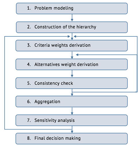
Fig. 4. Algorithm of the AHP
Steps 3, 4, 5, 6 represent the numerical procedure (so-called multiple criteria aggregation procedure). Pairwise comparisons are used to derive relative importance (weights) of general criteria with respect to their impact on the overall goal, then the weights of the secondary with respect to the general, ternary with respect to the secondary and so on until weights of all the criteria are defined. In step 4, weights of the alternatives are derived from the pairwise matrices. When weights of all the elements of the hierarchy are obtained, inconsistency in judgments should be checked. If there are some very inconsistent matrices, pairwise comparisons for them should be repeated, hence, the expert returns either to step 3 or to step 4.
If the expert is satisfied with the obtained result, then the procedure for synthesizing of local priorities across all criteria to the global priorities is launched. The expert uses distributive mode or ideal mode depending on the problem and his aim. Robustness of the result is tested in step 7. Effective decision making process have to include sensitivity analysis of the results.
2.3. Problem modeling
Problem modeling stage is undoubtedly one of the most important and less formalized phases of a solution of every decision problem. Two different problem structures may lead to two different alternatives rankings [14].
Hierarchical structure of the criteria is one of the AHP’s advantages. It should be built in compliance with principle of hierarchic composition (axiom 3 in [12]), at the same time the analytic should aim to build a hierarchy in which all criteria at one level have about the same number of the subcriteria. Several scientists have noticed that criteria with a large number of subcriteria tend to receive more weight than when they are less detailed.
2.4. Fundamental scale
The AHP has an advantage of permitting quantitative as well as qualitative criteria. In order to use qualitative criteria, values thereon must be somehow converted into numbers. Apart from that, even if everything in this world were measurable, people would still need to compare values measured on the different scales.
Table 1. Fundamental scale
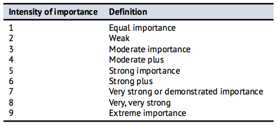
Therefore, fundamental scale of 1-9 is used in the AHP table 1. Saaty advises [7] to use the scale even for the quantitative criteria when the exact values are known. However, every analytic decides it himself.
Numerous articles and papers have been written concerning the scale. Among the possible drawbacks researches pointed out absence of zero, lack of sensitivity. However, despite of other proposed scales, the vast majority of the applications use the 1-9 scale. Besides, it is very difficult to verify whether the scale is effective or not. The choice of the scale depends on the analytic and the decision problem [1].
2.5. Pairwise comparisons
Instead of direct allocation of weights, relative verbal
judgements are used in the AHP. The expert constructs a square matrix where
rows and columns correspond to the alternatives ![]() . His
main task is to answer the question “how many times does the element in the
column on the left dominate the element in the row on top with regard to the
criterion?”.
. His
main task is to answer the question “how many times does the element in the
column on the left dominate the element in the row on top with regard to the
criterion?”.
This method is now called pairwise comparisons and it has been used long time before the AHP by psychologists. The scientists argue that it is easier to compare only two alternatives at a time. Apart from that, pairwise comparisons method is the procedure that gives the opportunity to use the ratio scale and get rid of physical units in the AHP.
Pairwise comparisons ![]() can
be arranged in a positive reciprocal matrix:
can
be arranged in a positive reciprocal matrix:
|
|
(1) |
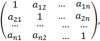
where ![]() is
the dominance of an object
is
the dominance of an object ![]() over
an object
over
an object ![]() with
respect to a criterion
with
respect to a criterion ![]() .
.
Elements of the matrix ![]() are
defined by the following entry rules:
are
defined by the following entry rules:
1. If ![]() , then
, then
![]() .
.
2. If objects
![]() and
and ![]() are
equally important then
are
equally important then ![]() ; in
particular,
; in
particular, ![]() for
all
for
all ![]() .
.
One of the main drawbacks of the method is that the number
of comparisons needed dramatically increases when a new criterion is
introduced. For a set of ![]() elements the number of pairwise
comparisons requested is
elements the number of pairwise
comparisons requested is ![]() ,
whereas the minimum number is
,
whereas the minimum number is ![]() judgements. According to some experts,
50% of the judgements are redundant and only necessary to check consistency.
Besides, sometimes the expert may not have formed a strong opinion on a particular
judgement, it is meaningless to force him to guess. In this case, the empty
cells may be filled using one of the following methods: calculation of missing
comparisons, starting rules, stopping rules [14].
judgements. According to some experts,
50% of the judgements are redundant and only necessary to check consistency.
Besides, sometimes the expert may not have formed a strong opinion on a particular
judgement, it is meaningless to force him to guess. In this case, the empty
cells may be filled using one of the following methods: calculation of missing
comparisons, starting rules, stopping rules [14].
The second disadvantage of the method is that the order in which comparisons are entered in the matrix may affect the subsequent judgements. In conclusion, it is important to note that not reciprocal matrices can be used as well. However, such cases are very rare and not considered in this paper.
2.6. Priorities derivation
Having recorded all quantitative judgements ![]() with
respect to a criterion
with
respect to a criterion ![]() about
alternatives
about
alternatives ![]() , in
other words, having filled in the pairwise comparison matrix
, in
other words, having filled in the pairwise comparison matrix ![]() , the
problem is how to create a set of numerical weights
, the
problem is how to create a set of numerical weights ![]() for
all
for
all ![]() .
.
For the further work we need to define what terms consistency and transitivity mean.
A matrix is said to be consistent, if
|
|
(2) |
A matrix is said to be transitive, if
|
|
(3) |
It is evident that expressions (2) and (3) always hold in case of a quantitative criterion. Moreover, a consistent matrix is always transitive. Thus, a question arises, in case of a qualitative criterion should the matrix satisfy (2) and (3), only (3) or neither of these two expressions? These questions laid the foundation of ongoing debates among the researchers. Saaty and his followers [1] support right eigenvector method for the priorities derivation, while Fichtner and several other believe that geometric mean is the most justified method.
Saaty states [7] that our world is inconsistent by its nature, thus, only minimum consistency is required to derive meaningful priorities. As for transitivity, in order to prove that the expression (3) should not necessary hold true Saaty gives the following example. In sports, team A beats team B, team B beats team C, but team C beats team A. Transitivity is violated but this situation can actually happen in the real world.
2.6.1. Right eigenvector
Right eigenvector method was proposed by Saaty in his first
publications [7]. Vector of priorities is derived here by solving the
eigenvalue problem ![]() or
or
|
|
(4) |
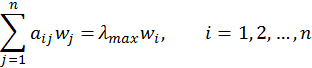
where ![]() is
obtained by solving the characteristic equation
is
obtained by solving the characteristic equation ![]() ,
, ![]() is the identity
matrix.
is the identity
matrix.
Fichtner wrote in [16] that “our mind may be a good
measurement device for priorities, it is certainly not the best one”. Besides,
we cannot avoid rounding errors using the 1-9 scale. Therefore, the equation ![]() have
to be supplemented by a perturbation factor
have
to be supplemented by a perturbation factor ![]() :
:
|
|
(5) |
In general, the perturbation factor is near 1. Let us substitute (5) in (4):
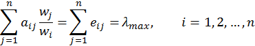
If there were no perturbation ![]() , i.e.
consistent case, the maximum eigenvalue of the matrix
, i.e.
consistent case, the maximum eigenvalue of the matrix ![]() would
be equal to the dimension of the matrix
would
be equal to the dimension of the matrix![]() (the
number of objects compared).
(the
number of objects compared).
Thus obtained vector depends a lot on the problem statement and, generally speaking, the right eigenvector is not necessary equals to the left one.
2.6.2. Geometric mean
The most used alternative to right eigenvector is geometric
mean which is also known as the logarithmic least squares method. Geometric
mean of the ![]() th row in the pairwise matrix is used as
the priority of the
th row in the pairwise matrix is used as
the priority of the ![]() th object.
th object.
In consistent case, ![]() and
the geometric mean of the
and
the geometric mean of the ![]() th row is
th row is ![]() .
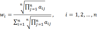
Normalized geometric mean is
.
Normalized geometric mean is
|
|
(6) |
In the general case, ![]() ,
thus, the vector derived by minimizing the multiplicative errors
,
thus, the vector derived by minimizing the multiplicative errors
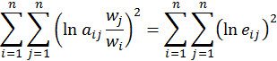
The solution of this problem is given by a normalized expression (6).
One of the main advantages of geometric mean is that it can be easily calculated by hand. Besides, geometric mean of rows and columns provide the same ranking, that means there is no right and left inconsistency.
2.7. Consistency
Deviation of a maximum eigenvalue ![]() from
the dimension of the pairwise matrix
from
the dimension of the pairwise matrix ![]() is used in [7] to measure inconsistency.
It allows to evaluate the obtained result. Consistency index:
is used in [7] to measure inconsistency.
It allows to evaluate the obtained result. Consistency index:
![]()
Inconsistency is considered a tolerable error in
measurements only when the ratio is in the range from ![]() to
to ![]() for
for ![]() and larger matrices,
from
and larger matrices,
from ![]() to
to ![]() for
for ![]() matrices, from
matrices, from ![]() to
to ![]() for
for ![]() matrices. These referential
values were obtained by averaging 500 results of 500 hundred simulations [7].
matrices. These referential
values were obtained by averaging 500 results of 500 hundred simulations [7].
2.8. Aggregation
Having derived all local priorities, the problem now is to
synthesize the weights across all criteria in order to determine the global
priorities. Linear aggregation is used for this purpose in the historical AHP
(now is called distributive mode). The weight of an object in the ![]() th level of the
hierarchy is multiplied by the weight of its parent object:
th level of the
hierarchy is multiplied by the weight of its parent object:
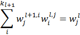
In this mode, the obtained weights sum to unity ![]() ,
thus, the aggregation procedure is recursive across the whole hierarchy.
,
thus, the aggregation procedure is recursive across the whole hierarchy.
In 1983 Belton and Gear in [17] provided an example that an introduction of a copy of an alternative can lead to changes in the ranking in distributive mode. In order to avoid this phenomenon, ideal mode was developed. Both of these methods are used now.
The expert should choose distributive mode if there is
dependence among the alternatives. In other words, alternatives from the set ![]() form
a closed system. In a closed system an amount of resources is fixed and
limited, for instance, allocation of a company’s budget or distribution of
votes among the election candidates.
form
a closed system. In a closed system an amount of resources is fixed and
limited, for instance, allocation of a company’s budget or distribution of
votes among the election candidates.
Let us consider the example about the company in more detail. Assume, in the beginning the company has two projects and the budget is allocated among them. If a new project is introduced it may lead to the rank reversal, i.e. one of the two initial projects will receive less money or will not receive any money at all. In this case, rank reversal phenomenon is not only possible but maybe is also desirable.
The expert should choose ideal mode if the alternatives are sufficiently distinct from each other. In contrast to distributive mode, in ideal mode a weight of an alternative with respect to each criterion is divided not by the sum of the weights of the all alternatives but by the largest value among them. In terms of systems science, ideal mode is used in open systems, i.e. in systems where the amount of resources is unlimited.
Ideal mode aims to obtain the single best alternative regardless of what other alternatives there are. Resulting priorities are measured on an interval scale and not on a ratio scale. Note that sometimes a product of an interval scale is meaningless, for instance, natural resource allocation.
3. Analysis of the AHP procedures
The following procedures form the essence of the AHP:
1. pairwise comparisons used to transform values measured on a physical scale into dimensionless numbers and to obtain weights of criteria and alternatives;
2. measurement of inconsistency using consistency index of pairwise matrices;
3. weights synthesis across all criteria using linear aggregation.
The main purpose of this chapter is to analyze how the
procedures mentioned above affect the final ranking of the alternatives. In
order to perform this analysis, calculations for ![]() matrices were
carried out.
matrices were
carried out.
3.1. Comparison of eigenvector and geometric mean methods for deriving priorities
An expert has to answer one question before making a choice between eigenvector and geometric mean. The question is “should the transitivity property hold true?”. If we consider the AHP as a framework, an approach for solving decision making problems, then the expert should have an opportunity to choose a method for deriving a priority vector from a pairwise matrix. If the expert believes that transitivity is essential, then he should use geometric mean. Otherwise, eigenvector is the way.
In case of consistent matrices, the weights obtained using eigenvector
equal to the weights obtained using geometric mean. Thus, inconsistent
transitive pairwise matrices are the object of the research. In order to assess
transitivity of a pairwise matrix, transitivity coefficient is used
[18]. Its calculation is based on a special matrix ![]() that
has to be built in accordance with the following rules:
that
has to be built in accordance with the following rules:
1. If ![]() is an
element of a pairwise matrix
is an
element of a pairwise matrix ![]() , then
the corresponding element of the matrix
, then
the corresponding element of the matrix ![]() .
.
2. If ![]() , then
, then
![]() ;
;
3. If ![]() , then
, then
![]() .
.
Violation of the transitivity property means that there are loops in the pairwise matrix. We can assess transitivity counting loops of length tree in strict order binary relations. Thus, transitivity coefficient [18]:
![]()
where ![]() is a number of loops of length three in
the corresponding graph,
is a number of loops of length three in
the corresponding graph, ![]() is
the maximum possible number of loops of length three.
is
the maximum possible number of loops of length three.
Transitivity coefficient is in the range of ![]() , at
that,
, at
that, ![]() implies perfect transitivity,
implies perfect transitivity, ![]() otherwise.
otherwise.
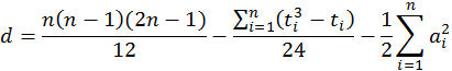
If the expert uses not only strict order binary relations but also indifference relations, then the transitivity coefficient is given by
|
|
(7) |
|
|
(8) |
where
![]() –
number of rank repetitions;
–
number of rank repetitions; ![]() –
number of arcs coming out of the
–
number of arcs coming out of the ![]() th vertex.
th vertex.
In order to compare eigenvector and geometric mean methods for deriving priorities from pairwise matrices, dependence of correlation coefficients between original and consistent matrices from transitivity coefficient of the original matrix was analyzed.
Matrices ![]() based
on one of the two descried methods were constructed. The following formula was
used to calculate correlation between elements of the original matrix
based
on one of the two descried methods were constructed. The following formula was
used to calculate correlation between elements of the original matrix ![]() and
elements of the consistent matrix
and
elements of the consistent matrix ![]() :
:
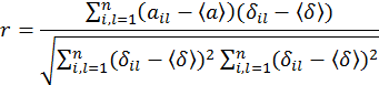
The following figures were built using formulas (7) and (8).
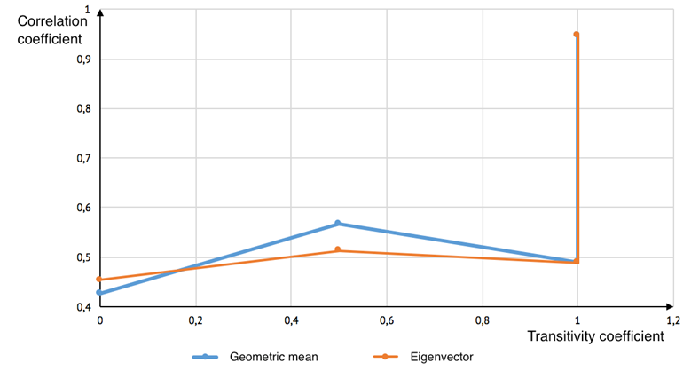
Fig. 5. Dependence between correlation coefficient and transitivity coefficient for 4×4 matrices
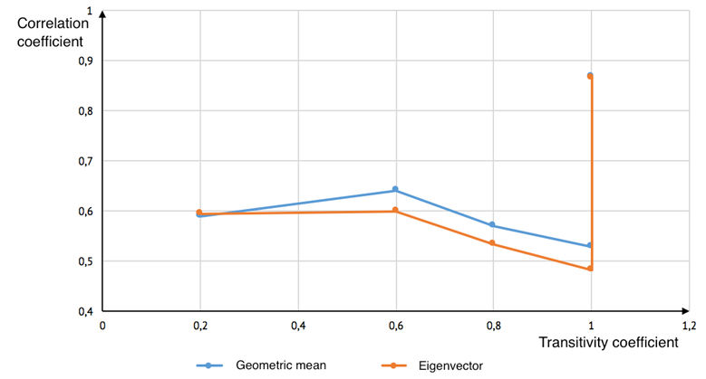
Fig. 6. Dependence between correlation coefficient and transitivity coefficient for 5×5 matrices
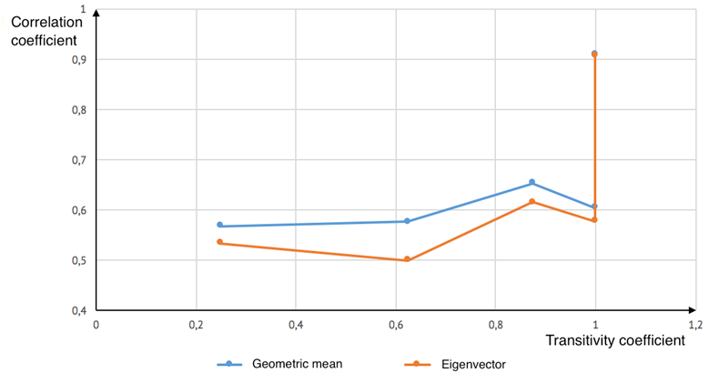
Fig. 7. Dependence between correlation coefficient and transitivity coefficient for 6×6 matrices
The obtained results show that geometric mean is a more justified method for deriving priorities than eigenvector. Correlation coefficient for geometric mean increases with rising inconsistency (decreasing transitivity coefficient). Such dependence does not hold true for eigenvector.
However, since transitivity coefficient is discrete, dependence of correlation coefficient while transitivity coefficient equals to unity war performed.
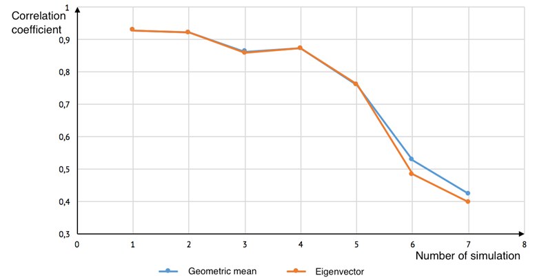
Fig. 8. Dependence of correlation coefficient while transitivity coefficient T=1
The result shows that the matrices based on geometric mean reflect initial data more precise than the matrices based on eigenvector, because in the first case correlation coefficient is closer to unity.
In spite of the fact that numerous researches testify clearly for geometric mean over eigenvector, there is no clear difference between these two methods in practice [19]. It is important to note that 18 different methods have been proposed to derive priorities [20] but 15 are equivalent and based either on one of the methods described above or on arithmetic mean of rows.
3.2. Analysis of consistency index
In order to analyze eigenvalue as a measure of inconsistency, research of dependence of correlation coefficient from eigenvalue was performed. During the research transitivity coefficient was kept constant T=1.
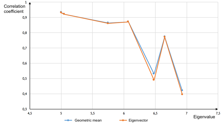
Fig. 9. Dependence of correlation coefficient from the eigenvalue while transitivity coefficient T=1
Fig. 9 shows that dependence between correlation coefficient and eigenvalue is not monotonous. Hence, its usage as a measurement of inconsistency is not valid. Apart from that, it was shown that consistency index allows contradictory judgements in matrices [21] and sometimes rejects reasonable matrices [22].
3.3. Analysis of linear aggregation
It was shown, that ideal mode is not ideal and that it is sometimes also a subject to rank reversal. Linear aggregation is the reason of this phenomenon, thus, the phenomenon is not unique only to the AHP. The final relative scale depends on the original set of alternatives due to the normalization.
Any alterations in the initial set of alternatives ![]() (when
a new alternative is added or removed) lead to the corresponding alterations
in weights. If weights change, the final scale also changes. Thus, the
resulting priorities depend on the initial set of alternatives. This is the
reason why rank reversal phenomenon occurs.
(when
a new alternative is added or removed) lead to the corresponding alterations
in weights. If weights change, the final scale also changes. Thus, the
resulting priorities depend on the initial set of alternatives. This is the
reason why rank reversal phenomenon occurs.
Since additive aggregation is the only way to synthetize
weights of known objects in the AHP [23], applicants can avoid this phenomenon
adding an ideal alternative for each criterion ![]() . One
should add this ideal alternative (it might not be real) before filling the
pairwise matrices.
. One
should add this ideal alternative (it might not be real) before filling the
pairwise matrices.
4. Sensitivity analysis
Sensitivity analysis is a prerequisite for model building since it determines the reliability of the model through assessment of uncertainties in the simulation results [2]. Visualization has been widely used in this step of the AHP [2,6,24]. It is appropriate to consider visualization in natural resource management separately from all other problems.
4.1. Tasks of sensitivity analysis and usage of visualization for solving them
Some problems of decision making may be inherently unstable. Different initial conditions may lead to completely different final rankings. Thus, to obtain the resulting weights one should conduct sensitivity analysis that can help the expert:
1. To assess the impact of changes in weights of objects on resulting priorities of alternatives.
2. Identify the critical elements of the decision.
3. Test the robustness of the obtained decision.
4. Generate scenarios of possible rankings of decision alternatives under different conditions.
5. Help the experts involved in a decision to reach a consensus.
6. Answers to ‘‘what if’’ questions.
Let us consider all these tasks one by one. In order to provide some illustrations, a decision support software MakeItRational [25] was used.
To assess the impact of changes in weights of objects, MakeItRational offers a special element of the graphical user interface that is represented in fi. 10. The weight of criterion (a circle) is divided by weights of the corresponding subcriteria (sectors of the circle).
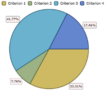
Fig. 10. Criteria weights
The expert can reduce or increase areas of sectors, thus, he will reduce or increase the weight of the corresponding criterion. At the same time, he can observe changes in resulting priorities of the alternatives. If insufficient changes in areas lead to sufficient changes in resulting priorities, this criterion can be said to have a big impact on the final ranking.
Fig. 11 provides important information on critical elements of the decision. Critical elements are the elements that contribute a lot in the final ranking. Apart from that, the expert might be also interested in finding objects that do not contribute at all or identify alternatives, high resulting priority of which caused only by one criterion.
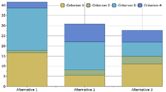
Fig. 11. Aggregated ranking
Every object is represented by its own column in fig. 11.
Columns consist of multicolored rectangles. A number of the rectangles is the
number of criteria on the same level of the hierarchy. If we are comparing
alternatives with respect to criteria on the ![]() th level, heights of
rectangles are weights of the alternatives on the
th level, heights of
rectangles are weights of the alternatives on the ![]() th level multiplied by
weights of the corresponding criteria on the
th level multiplied by
weights of the corresponding criteria on the ![]() th level.
th level.
Regarding the example in fig. 11, note that rectangles for “Criterion 2” (green color) are not high. Even if we delete these green rectangles the first column will be the highest, the second column will be higher than the third. Hence, “Criterion 2” does not contribute a lot in the final ranking.
The expert can test the robustness of the obtained decision using fig. 12. The result is said to be robust if the ranking does not change due to small modifications of the input data, otherwise it is sensitive.
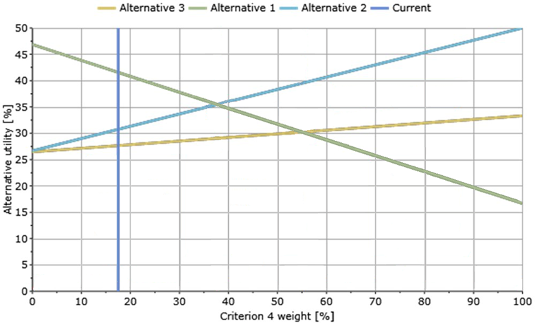
Fig. 12. Visual representation of alternatives to test the robustness
Green, light blue and yellow lines correspond to weights of “Alternative 1”, “Alternative 2” and “Alternative 3” with respect to “Criterion 4”. Blue vertical line “Current” shows the weight of “Criterion 4” and ranking of alternatives at the moment. A point of intersection of “Current” and horizontal coordinate axis allows to know the exact weight of “Criterion 4” (18% in this case).
One can obtain the final ranking by finding points of intersection of “Current” and lines for alternatives 1, 2, 3. The most preferable alternative is the alternative the point of intersection of which is the highest. The second preferable is the alternative the point of intersection of which is the second highest and so on. The final ranking in fig. 12 is “Alternative 1”, “Alternative 2”, “Alternative 3”.
The expert can change the weight of “Criterion 4” moving the blue line to the left if he wants to reduce it or to the right if he wants to increase it. However, the ratio between the rest criteria will remain constant. For instance, if “Criterion” 1, 2, 3 have weights 2%, 40%, 40% (the ratio is 1:20:20), then an increase of the weight of “Criterion 4” to 59% will lead to the fall of the weights of “Criterion” 1, 2, 3 to 1%, 20%, 20%.
The similar analysis might be conducted for the remaining criteria. Sometimes not enough information about the objects have been collected, sometimes people make mistakes. Sensitivity analysis allows to observe impact of changes in initial data to the final ranking not filling the pairwise matrices again.
Not everything can be predicted from the beginning (for example, earth phenomena). Hence, generation of different possible rankings scenarios under different conditions is needed. If the weight of “Criterion 4” rises by 30% in fig. 12 then the expert will observe the rank reversal. The most preferable alternative in that case will be “Alternative 2”.
Possibility of group work is an important advantage of the AHP. However, it is very difficult to avoid controversies and disagreements in this case. Sensitivity analysis can provide some understanding why different results were obtained and help the experts involved in a decision to reach a consensus.
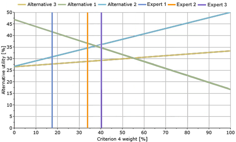
Fig. 13. Sensitivity analysis in group decision making
In fig. 13 (made not using MakeItRational) three experts participate in decision making. The blue line represents the ranking obtained by "Expert 1", orange line – "Expert 2", violet line – "Expert 3". According to fig. 13, "Alternative 1" is the most preferable to the first and second experts, while "Expert 3" has another best alternative – "Alternative 2".
The weight of "Criterion 4" is the main cause of this difference in the final ranking. Despite the fact that "Expert 1" and "Expert 2" obtained the same final rankings and "Expert 2" and "Expert 3" did not, the difference between weights of "Criterion 4" in the first case is more than two times bigger than in the second. Thus, the situation in fig. 13 is ambiguous, the DM has to decide which weight of "Criterion 4" is the most possible. If the weight of "Criterion 4" is estimated to be in a range of 30-40%, then the result is sensitive.
It is important to note that lines for the alternatives depend not only on the weight of "Criterion 4" but also on weights of the remaining criteria. If the weights of the criteria varied from expert to expert, then the slope angles of the lines for alternatives would be different. In general, there would be three different lines per every alternative.
Fig. 12 can be also used for answering to "what if" questions. An example of a simple "what if" question is "what will happen if "Criterion 4" has a bigger weight?". Let us answer it. Alternatives 1 and 2 will have the same ranking when the weight of "Criterion 4" is about 38% (the vertical line will occupy the place of the left red dotted line), since the blue, green and light blue lines will intersect at one point. The point is circled on the left.
If the weight of "Criterion 4" is in the range of 38-55%, the final ranking will be "Alternative 2", "Alternative 1", "Alternative 3". If the weight is increased, then the final ranking will be "Alternative 2", "Alternative 3", "Alternative 1".
Fig. 12 concludes a lot of information about resulting priorities of the objects in respect to changes in the weight of "Criterion 4". MakeItRational allows setting up the values with a 0.1% step. Hence, 1001 value of resulting priorities with respect to “Criterion 4” are pointed in fig. 12.
In order to provide visualizations, a decision support software MakeItRational was used in this chapter. However, it should be noted that several other support packages that allow the analyst to use the AHP and to conduct sensitivity analysis have been developed. For example, 123AHP [26], Creative Decisions Foundation [27], Decision Lens [28], Expert Choice [29], ????? [30] and several other.
4.2. Visualization in GIS
A very important characteristic of natural resource management tasks is that visualization can be already used in them on the problem modeling step. In [6] the AHP is applied within a GIS to create suitability maps for sand and gravel mining in the vicinity of Frankfurt (Germany). Five criteria of one level of a hierarchy were considered: water protection zones, distance buffers around existing settlements, the thickness of the overburden, the thickness of sand and gravel deposits and soil productivity.
The input data for every criterion is represented as a map, different colors are used to show different values of the criteria. For example, for “soil productivity” criterion level of the soil productivity can be measured with values in a range of 0-6. We can denote numbers 0, 1, 2 with 7 different colors fig. 14.
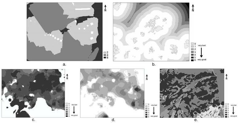
Fig. 14. Representation of the input data: a. criterion “water protection zones”; b. criterion “distance buffers around existing settlements”; c. criterion “the thickness of the overburden”; d. criterion “the thickness of sand and gravel deposits”; e. criterion “soil productivity”
Having collected all input data and represented it as it is shown in fig. 14, the problem is to assign every criteria a set of weights and to perform linear aggregation. After that, the expert slightly modifies the weights in order to tests the robustness of the obtained decision fig. 15. As the result, three spots were chosen. The spots are outlined by black circles.
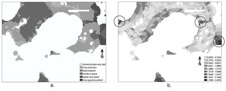
Fig. 15 Sensitivity analysis for the sand and gravel mining example: a. the first set of the criteria weights; b. the second set of the criteria weights
Another example of how the AHP can be used in GIS is presented in [2]. Land suitability assessment for potential irrigated agriculture in Queensland (Australia) was hold. In order to conduct sensitivity analysis, the original weights for the five different criteria from the base run were varied within a range of 20% provided that a 1% step was used for simulations. Thus, the experts obtained 40 summary tables that would be very difficult to analyze without visualization.
4.3. Approaches to sensitivity analysis and visualization in them
In [31] three different approaches to sensitivity analysis are described:
1. Numerical incremental analysis
In order to conduct sensitivity analysis in this case, the expert changes the input data. It leads to the corresponding changes in the final ranking. The obtained result can be represented graphically using different diagrams (for example, fig. 1).
This approach is implemented in the vast majority of AHP-based decision support systems. One should note here that these systems usually allow to modify only values on the first level of the hierarchy. Moreover, they do not allow more than one change at a time.
2. Simulation approach
This approach to sensitivity analysis is based on replacement of deterministic weights with stochastic. A similar approach was used in [24] to reach a good morphological state of a river. In order to evaluate the current situation of the river and to decide whether the further reparations are needed the hierarchy was designed fig. 16.
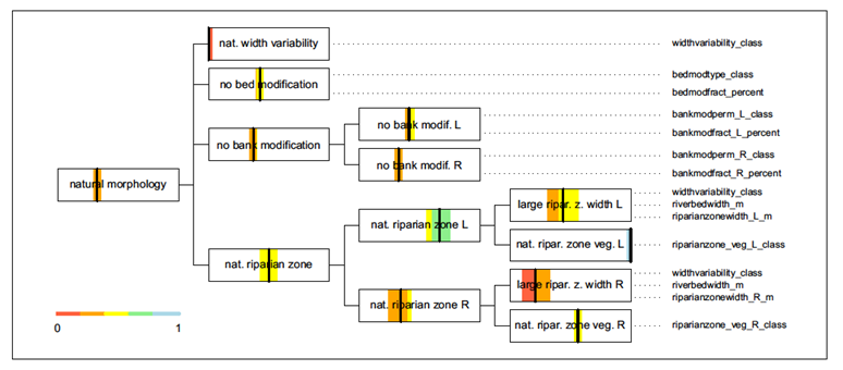
Fig. 16. The current morphological state of the river
A vertical line indicates the corresponding value on the scale between zero and unity along the horizontal extension of the box. Colored areas cover 95% quantile intervals, thus, representing uncertainty of the observations.
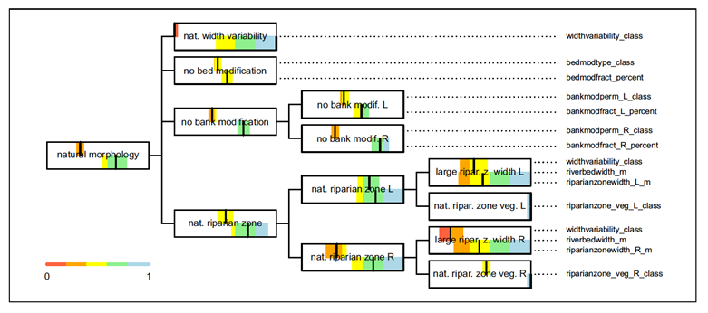
Fig. 17. Comparison between the current and a future state
The experts evaluated the future state that will be reached after implementation of the rehabilitation measures. A comparison between the two states was visualized by coloring the upper and lower parts of the nodes fig. 17. The upper part corresponds to the current state, the lower – to the future predicted state. This graphical representation allows the expert to compare alternatives while also representing uncertainty.
In the AHP, numerical incremental analysis and simulation approach can be done on three levels: weights, local priorities and comparisons.
3. Mathematical deduction method
This method is used when simple closed-form expressions can
describe the relationship between input and output data. Robustness of the
obtained decision estimates here using sensitivity coefficient. Several
different approaches to calculate sensitivity coefficient ![]() have
been developed. More information can be found in [24]. One of the simplest
formulas is [32]
have
been developed. More information can be found in [24]. One of the simplest
formulas is [32]
![]()
where ![]() is
the smallest percent amount by which the current value must be changed such
that the ranking is reversed.
is
the smallest percent amount by which the current value must be changed such
that the ranking is reversed.
Note that visualization was used in all approaches to sensitivity analysis except the last one. Sensitivity coefficient that was discussed in mathematical deduction method is a cumulative index. Its informativeness is lower than informativeness of other graphical representation of data viewed in other methods.
In the formula for sensitivity coefficient ![]() – the
smallest percent amount by which the current value must be changed such that
the ranking is reversed, was used. This value can be also obtained from the fig.
12. It is difference between two values on the abscissa axis. One corresponds
to the point of intersection of abscissa axis and the right red dotted line,
another one – the point of intersection of abscissa axis and vertical blue line
“Current”.
– the
smallest percent amount by which the current value must be changed such that
the ranking is reversed, was used. This value can be also obtained from the fig.
12. It is difference between two values on the abscissa axis. One corresponds
to the point of intersection of abscissa axis and the right red dotted line,
another one – the point of intersection of abscissa axis and vertical blue line
“Current”.
5. Conclusion
In this paper, the AHP was discussed. The method helps to achieve a trade-off between mapping the real world and usability of the model and it has been widely used in the past. For example, in education, engineering, management, manufacture, politics and sport. The AHP follows people’s intuitive way of thinking and it allows hierarchical modeling of problems and possibility to use verbal judgements.
Chapters 1 and 2 were devoted to two fundamental decision making problems: rank reversal and measurement of inconsistency of judgements. It is important to note that decision making has combined engineering sciences and humanities. Thus, this might be the reason why the problems emerged.
The results of chapter 2 section 1 show that if transitivity property holds true then geometric mean method is a more justified method for deriving priorities than eigenvector. In this case, the expert should use correlation coefficient between initial and consistent matrices in order to assess pairwise matrices. In addition to it, transitivity coefficient is recommended.
A new alternative to ideal mode is proposed in chapter 2 section 1. In this method, weights of objects are normalized by dividing weights by the weight of an ideal object (object with the largest weight with respect to the criterion). Weights of alternatives will no longer depend on the initial set, thus, the rank reversal problem can be avoided.
Sensitivity analysis in the AHP was discussed in chapter 3 of this paper. Problems of natural resource management was considered separately, since GIS systems allow to visualize not only the results but also the input data. Visualization of dependence between input and output data can provide better insight into critical elements of the decision, create more realistic scenarios, test the robustness of the obtained result.
The visualization serves as an argumentation base for the final decision. It allows the expert to analyze huge amounts of tabular data within a limited amount of time. It is important to note that methods of visualization in decision making have received limited attention in the past. Further researches on that are required.
References
- Harker P.T., Vargas L.G. The theory of ratio scale estimation: Saaty’s Analytic Hierarchy Process. Management Science, 1987, Vol. 33, No. 11, pp. 1383-1403.
- Chen Y., Yu J., Shahbaz K., Xevi E. A GIS-Based Sensitivity Analysis of Multi-Criteria Weights, 18th World IMACS / MODSIM Congress, 2009.
- Stummer C.A., Kiesling E., Gutjahr W.J., Multicriteria decision support system for competence-driven project portfolio selection, International Journal of Information Technology & Decision Making, 2009, Vol. 8, No. 2, pp. 379-401.
- Pilyugin V., Malikova E., Pasko A., Adzhiev V. Nauchnaja vizualizacija kak metod analiza nauchnyh dannyh [Scientific visualization as method of scientific data analysis]. Scientific visualization, 2012, vol. 4, no. 4, pp. 56-70. [In Russian]
- Packham I.S.J., Rafiq M.Y., Borthwick M.F., Denham S.L. Interactive visualization for decision support and evaluation of robustness – in theory and in practice. Advanced Engineering Informatics, 2005, Vol. 19, pp. 263-280.
- Marinoni O., Hoppe A. Using the Analytical Hierarchy Process to support sustainable use of geo-resources in metropolitan areas, Journal of Systems Science and Systems Engineering, 2006, Vol. 12, No. 2, pp. 154-164.
- Saaty T.L. The Analytic Hierarchy Process: Planning, Priority Setting, Resource Allocation, McGraw-Hill, New York, 1980, – 290 ?.
- Subramanian N., Ramanathan R. A review of applications of Analytic Hierarchy Process in operations management, International Journal of Production Economics, 2012, No. 138, pp. 215-241.
- Kolesnikova S. I. Osobennosti ppimenenija linejnoj sveptki kpitepiev v metode parnyh sravnenij [Feature of Usage of Linear Convolution of Criteria in Method of Paired Comparisons]. Information technologies, 2011, no. 1 (173), pp. 24-29. [In Russian]
- Nogin V. D. Upposhhennyj variant metoda analiza iepaphij na osnove nelinejnoj sveptki kpitepiev [A simplified variant of the hierarchy analysis on the ground of nonlinear convolution of criteria]. Zh. Vychisl. Mat. Mat. Fiz., 2004, vol. 44, no. 7, pp. 1259—1268. [In Russian]
- Forman E.H., Gass S.I. The analytic hierarchy process – an exposition. Operations Research, 2001, Vol. 49, No. 4, pp. 469-486.
- Saaty T.L. Axiomatic foundation of the Analytic Hierarchy Process. Management Science, 1986, Vol. 32, No. 7, pp. 841-855.
- Roy B. Multicriteria Methodology for Decision Aiding. Springer Science & Business Media, 2013, 293 p.
- Ishizaka A., Labib A. Review of the main developments in the analytic hierarchy process. Expert Systems with Applications, 2011, No. 38, pp. 14336-14345.
- Saaty T.L. Response to holder’s comments on the analytic hierarchy process. Journal of the Operational Research Society, 1991, Vol. 42, pp. 909–929.
- Fichtner J. On deriving priority vectors from matrices of pairwise comparisons. Socio-Economic Planning Sciences, 1986, Vol. 20, No. 6, pp. 341-345.
- Belton V., Gear A. On a shortcoming of Saaty’s method of analytical hierarchies. Omega, 1983, Vol. 11, pp. 228–230.
- Eltarenko E.A., Krupinova E.K. Obrabotka jekspertnyh ocenok [Processing expert assessments]. NRNU MEPhI, 1982, 94 p. [In Russian]
- Saaty T.L. Vargas L.G. Comparisson of eigenvalue, logarithmic least squares and least squares methods in estimating ratios. Mathematical Modelling, 1984, Vol. 5, pp. 309-324.
- Cho E.A., Wedley W. common framework for deriving preference values from pairwise comparison matrices. Computers and Operations Research, 2004, Vol. 31, pp. 893–908.
- Kwiesielewicz M., van Uden. E. Inconsistent and contradictory judgements in pairwise comparison method in AHP. Computers and Operations Research, 2004, Vol. 31, pp. 713–719.
- Karapetrovic S. Rosenbloom E. A quality control approach to consistency paradoxes in AHP. European Journal of Operational Research, 1999, Vol. 119, pp. 704–718.
- Vargas L. Comments on Barzilai and Lootsma why the multiplicative AHP is invalid: A practical counterexample. Journal of Multi-Criteria Decision Analysis, 1997, Vol. 6, pp. 169–170.
- Reichert P., Schuwirth N., Langhans S. Constructing, evaluating and visualizing value and utility functions for decision support. Environmental Modelling & Software, 2013, Vol. 46, pp. 283-291.
- MakeItRational. URL: http://makeitrational.com (accessed 27.04.2016)
- 123ahp. URL: http://www.123ahp.com (accessed 08.05.2016)
- Creative Decisions Foundation. URL: http://www.creativedecisions.org (accessed 08.05.2016)
- Decision Lens. URL: http://decisionlens.com (accessed 08.05.2016)
- Expert Choice. URL: http://expertchoice.com (accessed 08.05.2016)
- Vibor. URL: http://www.ciritas.ru/product.php?id=10 (accessed 08.05.2016)
- Chen H., Kocaoglu D.F. A sensitivity analysis algorithm for hierarchical decision models. European Journal of Operational Research, 2008, Vol. 185, pp. 266-288.
- Triantaphyllou E., Sánchez A. A sensitivity analysis approach for some deterministic multi-criteria decision-making methods. Decision Sciences, 1997, Vol. 28, No. 1, pp. 151-194.