VERTEX SHADER FOR VISUALIZING A DEFORMABLE STRIP
Stepan Orlov*, Nikolay Shabrov
Peter the Great St. Petersburg Polytechnic University, Computer Technologies in Engineering Department
*Corresponding author E-mail: majorsteve@mail.ru, Phone: +7 911 923 2705, Fax: +7 812 552 7770
Contents
3 Approximating strip axis geometry
4. Approximating strip volume geometry
5. Approximating strip geometry at ends
6. Implementation of vertex shader
6.1. Examples of deformed strip visualization
Abstract
The paper is dedicated to the development of a vertex shader used to visualize a deformable strip. An approximation of strip geometry in the deformed state is proposed, taking into account the necessity to visualize magnified deformations. Importantly, the deformed state to be zoomed and visualized comes from the solution of elasticity problem considering small deformations. In this case, the zoomed deformed state needs to be defined carefully in order for it to look natural. Also, attention is paid to the approximation of geometry at strip ends, where the deformations are absent. The source code of the vertex shader is listed.
Keywords: deformable body visualization, deformable strip kinematics, exaggerated deformations, vertex shader, GLSL
1. Introduction
Early versions of OpenGL provided the way of visualization using the so called fixed pipeline [1]. Starting with OpenGL 2.0, vertex and fragment shaders can be used, making some parts of the fixed pipeline optional. Moreover, in some OpenGL editions (e.g., OpenGL ES), those optional parts of fixed pipeline no longer exist.
While the fixed pipeline is suitable for rendering geometry consisting of rigid bodies, this is not the case for deformable bodies. The problem with deformable bodies is that each vertex of a mesh representing body’s boundary surface needs to undergo a specific transformation in addition to model, view, and projection (MVP) transformation, and that the additional transformation is different at each vertex (i.e., cannot be formulated as a matrix-vector product with the matrix fixed for all vertices). GLSL vertex shaders are designed to solve exactly this kind of problem: transform each vertex separately. Section 2 briefly overviews existing approaches in this area.
This paper is dedicated to the development of a vertex shader for a particular case of deformable body — a thin 3D strips that experiences deformations of extension, torsion, and bending in one plane. This kind of deformable body appears in the modeling of continuously variable transmission (CVT) [2]. An essential part of the transmission is the chain consisting of rocker pins and plates (Figure 1). The chain contains about 1000 deformable plates, and they are visualized using the shader described in this paper (each plate is one deformable strip).
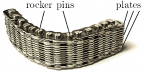
Fig. 1. CVT chain
The deformations of the strip result from a numerical simulation. Importantly, all deformations are considered small in the numerical models. However, the user typically wishes to see how the strips deform. This requires an exaggeration, or zooming, of actual deformations in order to make them visible. The zooming of deformations has to be done carefully in order to make the deformed body look natural. Sections 3, 4 describe how that can be done.
Forces and torques acting on a CVT chain plate are applied on its inner contour, where rocker pins are attached to it. Due to this, parts at ends of the plate do not deform (if we limit ourselves to the level of accuracy provided by the mechanical model of plate). As follows from our experience, it is important to take it into account when visualizing a plate with deformation zooming. Section 5 provides additional details on the kinematics of the end parts and shows relevant examples of visualization.
Section 6 discusses the implementation of a vertex shader for visualizing a deformable strip and shows examples of visualization of a strip for different deformed states using the final version of the vertex shader. Shader source code listing is presented.
Section 7 provides a short summary of the results.
2 Related work
Probably the first attempt to achieve visual local deformation on a surface dates back to 1978, when Blinn introduced [3] what now is known as bump mapping. Notice, however, that this technique does not actually imply any modification of surface mesh vertices.
Many works on the visualization of a deformable surface mesh started appearing much later, when vertex shaders became available on graphic hardware. Large number of papers in this area is related with many different requirements to be met, as well as many possible ways to describe the deformations. The simplest and most general way to specify the deformed mesh is to introduce the displacement vector at each vertex [4, 5]. The problem with this approach is that the data describing the deformation is as large as the vertex buffer itself. To reduce data transfer from CPU to GPU during animations, further steps need to be taken. One approach is to transfer data on a coarse mesh and then interpolate displacements on a finer mesh on the GPU [5]. Another approach is to compute the displacements on the GPU [6, 7], thus eliminating any data transfer for the deformed mesh data.
In many applications, the positions of vertices need to be computed without a complicated simulation — for example, due to the performance requirement. Therefore, there are approaches allowing to specify deformations using a relatively small amount of data and compute the displacement vector from that data in a vertex shader. One of the most popular among these approaches is the mesh skinning [8,9,10,11,12]. The basic idea is to specify the motion of several rigid bones of the skeleton and compute vertex positions from the configuration of the bones; the algorithm presented in [9] can also handle deformable bones.
Work [13] presents an approach to the visualization of deformed mesh using fragment shader; possible mesh deformations even include cuts.
There are applications where skeleton-based skinning is still too complex in terms of performance. For example, the rendering of grass requires a combined approach, where only parts of the scene close to the camera are rendered using a deformable mesh for individual grass blades [14]; more distant parts are rendered in a simpler way, e. g., as suggested in [15].
Other techniques to describe a deformed surface mesh exist, some based on textures. An interesting approach is presented in [16]; its visualization part can be thought of as a development of bump mapping.
In [17], vertex shaders are used to visualize B´ezier curves [18] and Catmull-Rom splines [19].
The approach to the deformed mesh visualization closest to the one presented here is described in [20]; it differs from ours in that the shape of the axis line is specified using a texture, and that rigid end parts are not considered.
3 Approximating strip axis geometry
We consider that the strip being visualized has a specific axial line, or axis. In the undeformed state, the axis is a straight line.
At each point of the axis, a cross-section of the body is defined. In the undeformed state, the cross-section is the intersection of the strip body with the plane perpendicular to the axis and passing through the point on the axis.
Let us introduce two points on the axis, A0 and A1. The part of the strip between cross-sections at these points is considered to be the “middle” of the strip. Other two parts are considered to be the “ends” of the strip. The ends are always considered to be undeformed, which is discussed in Section 5. The middle of the strip experiences deformations.
The distance between points A0 and A1 is denoted by l in the undeformed state, and by L in the deformed state. We also introduce parameter p on the axis. It is the signed distance, divided by l, from point A0 to the specific point on the axis, counted towards point A1, in the undeformed state. The p parameter is dimensionless and varies from zero to one in the middle part of the strip (between points A0 and A1) and is outside the range [0, 1] at strip ends.
Figure 2 illustrates the above considerations.
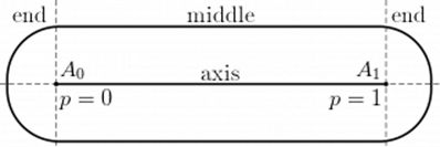
Fig. 2. Axis and axial coordinate p in strip body
The deformed state of the strip (its middle part) can be described in terms of extension along the axis, torsion about the axis, and bending in one plane perpendicular to the axis. Besides, the position and orientation of the strip in the object Cartesian coordinate system should be specified. To do that, first let us notice that the strip median surface always remains close to the OXY plane of the object coordinate system, and the orientation of strip in the plane can be arbitrary. Therefore, it is convenient to specify positions R0,0 and R0,1 of points A0 and A1, respectively, in the deformed state.
Our goal in this section is to define the radius-vector R0(p) of a point on the axis in the deformed state, for any p ∈ [0, 1]. Let us represent it as follows:
|
|
(1) |
where ![]() 0 is a point on straight line that
would be the deformed strip axis in the absence of bending:
0 is a point on straight line that
would be the deformed strip axis in the absence of bending:
|
|
(2) |
Therefore, the displacement vector u⊥ describes the deflection of the axis from straight line.
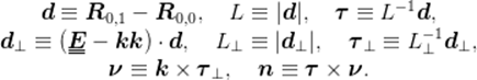
Next we need to define the orientation of strip cross-section axes, considering the case of no torsion and no bending at first. To do that, denote the direction vectors of the axes OX, OY , OZ of the object coordinate system by i, j, k, respectively, and introduce four more unit vectors, τ, τ⊥, ν, and n, as follows:
|
|
(3) |
Notice that E is the identity tensor of rank 2
in 3D space, and E -kk is the projector onto the
plane OXY (we use the direct tensor notation, see, e.g., appendix I
in [21]).
The meaning of these vectors is quite simple: τ is the unit
vector of the direction of line ![]() 0(p); τ⊥ is the normalized
projection of τ onto the plane OXY , ν
is a vector in the plane OXY perpendicular to τ, and n
is the normal vector to the strip median plane, in the case of no torsion and
no bending. The vectors are shown in Figure 3.
0(p); τ⊥ is the normalized
projection of τ onto the plane OXY , ν
is a vector in the plane OXY perpendicular to τ, and n
is the normal vector to the strip median plane, in the case of no torsion and
no bending. The vectors are shown in Figure 3.
Fig. 3. Vectors determining strip orientation (no bending and torsion)
Notice that (τ⊥,ν,k) is an orthonormal right-handed basis, as well as (τ,ν,n). The second basis is rigidly connected with the strip, in the case of no torsion and no bending; it can be obtained from (i,j,k) by applying the sequence of rotations P (βν) ⋅ P (αk). The rotation angles are as follows:
|
|
(4) |
When using notation P (ψm), we mean that P is the rotation tensor corresponding to the finite rotation vector ψm. If |m| = 1, the rotation tensor is given by the following Euler formula [21, p. 434]:
|
|
(5) |
The next step is to introduce the torsion, which is done by linearly interpolating the torsion angle φ through its values φ0, φ1 at p = 0, p = 1, respectively
|
|
(6) |
and introducing the rotation of strip cross-section about the axis, P (φτ). Applying that rotation to (τ,ν,n) results in the new basis (τ,νφ,nφ) — see Figure 4:
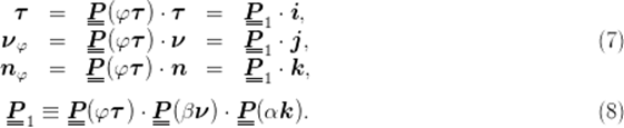
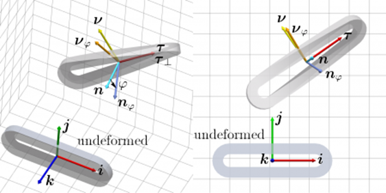
Fig. 4. Vectors determining strip orientation (torsion and no bending)
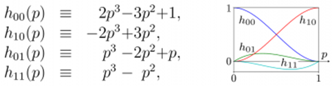
Finally, the bending needs to be taken into account. With no relationship with mechanics, we assume that the displacement u⊥ is parallel to nφ. The magnitude of the displacement can be computed using two of four Hermitian cubic polynomials:
|
|
(9) |
so that the displacement vector u⊥ takes the form
|
|
(10) |
Notice that the strip axis remains straight as soon as u0′ = u1′ = L-1d z.
4. Approximating strip volume geometry
To define the position of arbitrary point of the strip body in the deformed state, we make two assumptions typical for the Bernoulli — Euler beam model:
- Cross-sections remain rigid in the deformed state. For the visualization purposes, this is fairly reasonable.
- Cross-sections remain perpendicular to the axis in the deformed state (no shear). This is reasonable, since the Bernoulli — Euler beam model has actually been used to compute the bending deformations of the strip. In case of using, e.g., the Timoshenko beam model, this assumption should be dropped.
Consider an arbitrary point A of the strip body and the point Ap at the intersection of the axis and the cross-section containing point A. Due to the first of the above two assumptions, the position R of point A can be obtained using the rigid body kinematics formula:
|
|
(11) |
where
r, r0
are the positions of points A, Ap, resp., in the undeformed state;
x ≡ r -r0
determines is the position of point A in the cross-section;
![]() is a rotation tensor.
is a rotation tensor.
To compute the rotation of the cross-section due to the strip bending, let us use the no shear condition. In the case of small deformations, this means that the cross-section small rotation vector ϑ and the displacement vector u are connected by the following constraint:
|
|
(12) |
where (…)′ is the derivative with respect to
the arc length coordinate in the undeformed state, and γ is
the small deformation of extension and shear. Since the extension and torsion
deformations do not lead to shearing, we are free to treat the state with
extension and torsion applied as undeformed in (12).
That is, the axis in that “undeformed” state is determined by ![]() 0, and the
cross-section rotation tensor is P 1; the arc length
derivative is therefore computed as (…)′ = L-1d∕dp,
and axis tangent vector is
0, and the
cross-section rotation tensor is P 1; the arc length
derivative is therefore computed as (…)′ = L-1d∕dp,
and axis tangent vector is ![]() 0′ = τ.
0′ = τ.
Despite the fact that this constraint is actually employed in the linear theory used to compute small deformations of the strip, the non-linear no-shear constraint [22] has to be considered in order to construct the appropriate rotation of cross-section in the case of zoomed deformations:
|
|
(13) |
where Γ is the finite deformation of extension and shear, and θ is the finite rotation vector corresponding to the bending. In fact, the no-shear condition (13) simply gives the expression of θ through tangent vectors τ and T in the undeformed and deformed states:
|
|
(14) |
Computing the left hand side of the last equality in (14), we obtain
|
|
(15) |
The total rotation of strip cross-section is P 1 defined in (8), followed by the rotation due to the bending P (θ):
|
|
(16) |
Rotation matrices are computed most efficiently when the rotations are about the coordinate axes of the object coordinate system. For that reason, it is better to rearrange rotations in P 1 and exchange P__1 with P (θ) in (16). The following commutation formula can be obtained from (5) and used for that (see also [21]):
![]()
where Q is a rotation tensor, and P (ψm) is the rotation tensor determined by the finite rotation vector ψm. The final formula for the rotation of strip cross-section takes the form
![]()
where
|
|
(19) |
Practically, one can neglect the term φ′u⊥nφ in (15) without severely impacting visualization plausibility — that will yield θn = 0, and all rotations will be about fixed axes; but this is not necessary. An example is shown in Figure 5, where the same deformed strip is displayed twice: gray reflective surface is visualized correctly, and yellow translucent surface is visualized assuming φ′u⊥nφ = 0.
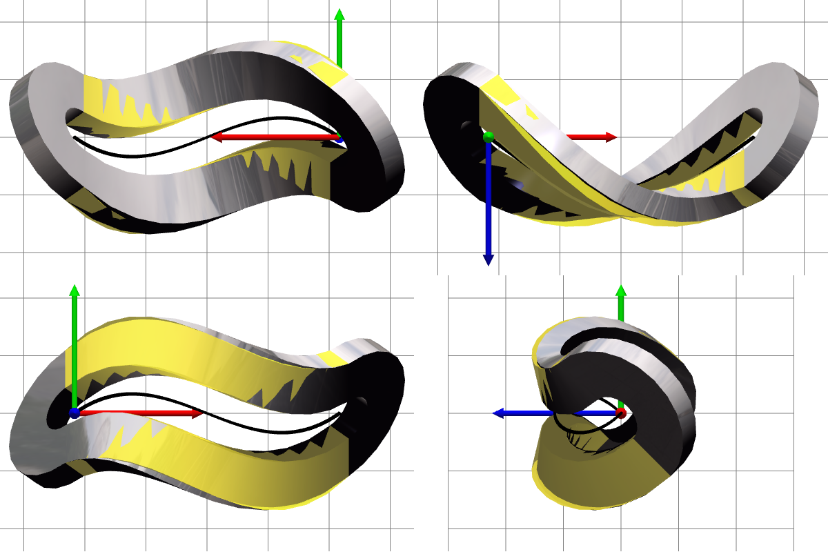
Fig. 5. Correct and simplified visualization of deformed strip.
To compute the position R of an arbitrary point of the strip in the deformed state, one should use formulas (3),(4),(6),(17),(7) for nφ only, (10),(2),(1),(15) to find θν, θn, (19), (18) and (11) in this order; some intermediate values can be optimized out.
5. Approximating strip geometry at ends
As already mentioned in Section 1, end parts of the strip (see Figure 2) do not deform. The reason is that all forces acting on the strip are concentrated at cross-sections p = 0 and p = 1. This means that the end parts remain rigid. In particular, strip axis at an end part remains straight; its slope must be the same as at the corresponding end of the main part, because the tangent to the axis is continuous. The orientation of the cross-section (i.e., the rotation tensor P ) is continuous too. From these simple considerations, the position R of arbitrary point A at an end part can be defined using the rigid body kinematics formula like (11):
|
|
(20) |
where R* and r* are the positions of a point at the end cross-section, p = 0 or p = 1, of the main part (e.g., the point on the axis), in the deformed and undeformed state, respectively; P * is the rotation tensor of that cross-section. See Figure 6.
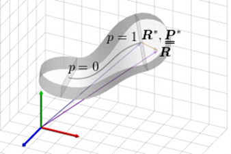
Fig. 6. Rigid body kinematics at end part of the strip
The importance of considering the ends parts rigid for the visualization is illustrated by examples in Figure 7: gray reflective surfaces are visualized with end parts considered rigid; yellow translucent surfaces are visualized without special treatment of the end parts, i.e., the same way as the middle part.
|
|
|
|
|
|
extension |
torsion |
bending |
all |
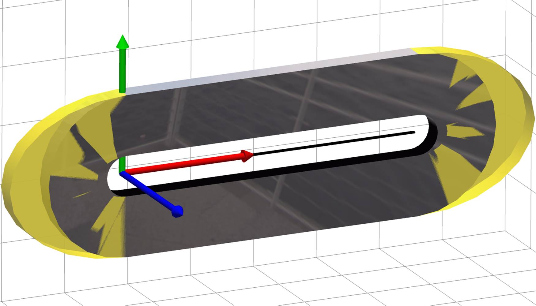
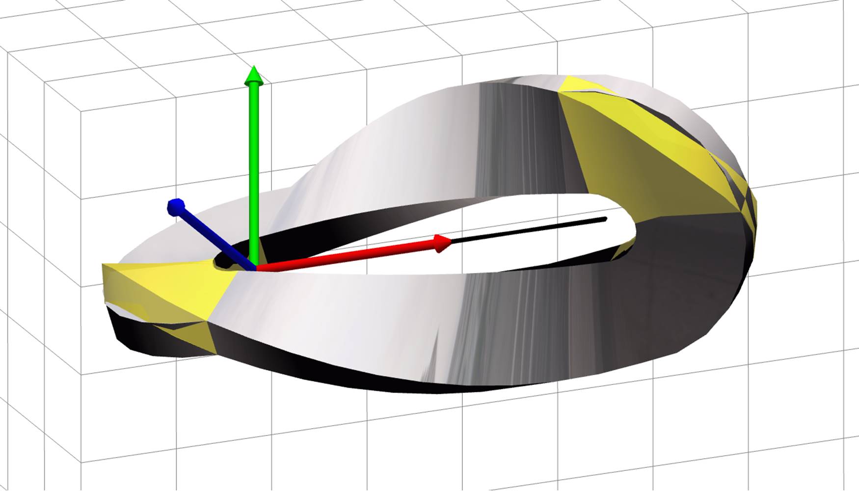
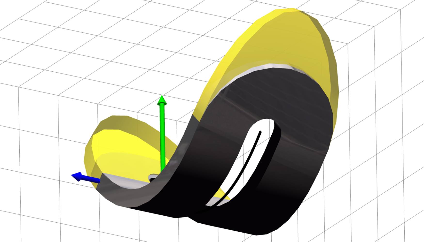
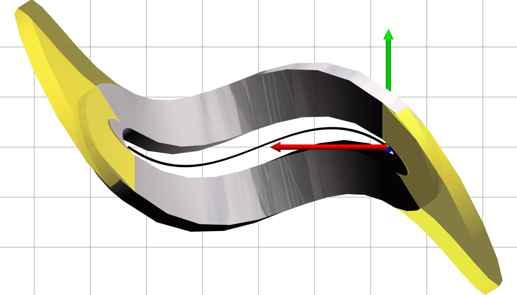
Fig. 7. Visualization of deformed strip with and without special treatment of the end parts
6. Implementation of vertex shader
This section describes the implementation of the vertex shader for deformable strip. The source code is written in GLSL version 1.20 [23], as follows from the #version directive in the listing below. This version has been chosen to enable the use of as early OpenGL standard version as possible (this is OpenGL 2.1), and in the same time to be able to use some convenient language features like implicit integer-to-float conversion and others.
Shader inputs are per-vertex attributes (3 coordinates x, y, z of vertex position vector r in object coordinate system, 3 surface normal vector coordinates, and 2 texture coordinates), and uniform values shared among all vertices being processed. The latter are common transformation matrices like model-view and others and arrays of values that determine the deformed state of the strip (those correspond to R0, u0′, φ0, R1, u1′, φ1 introduced in Section 3). In addition, uniform values include coefficients that determine a scalar field on the strip — there might be the need to visualize that field. Notice that the field is interpolated using Hermitian cubic polynomials (9).
Shader outputs are the vertex position (clip space coordinates), as well as a number of so called varying parameters at vertex (varying parameters are further interpolated at fragments and passed to fragment shader). These parameters are the eye coordinates of position and surface normal vectors, the texture coordinates, and the scalar field value.
When the shader processes a vertex belonging to an end part of the strip (see Section 5), it needs the point r* on the axis at the nearest end of middle part (p = 0 or p = 1), in the undeformed state — see (20). It seems that some piece of input data is missing, preventing us from being able to find r* for arbitrary vertex. However, there is a solution. If we require that the plane x = 0 is centered in the middle of undeformed middle part, p = 0.5, then we have x = -l∕2 at end p = 0, and x = l∕2 at end p = 1, so the undeformed length l of the middle part can be computed at almost any vertex, and at any vertex of each end part: l = x∕(p - 0.5). Therefore, r* can be computed as
|
|
(21) |
where plus in ± is taken at end p < 0 and minus — at end p > 1.
|
|
|
|
|
|
|
No deformation zooming |
100× deformation zooming |
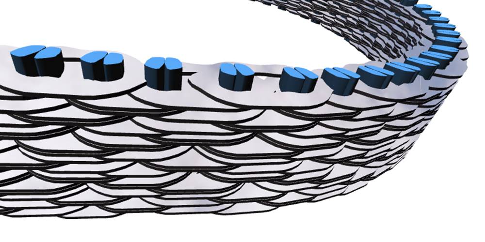
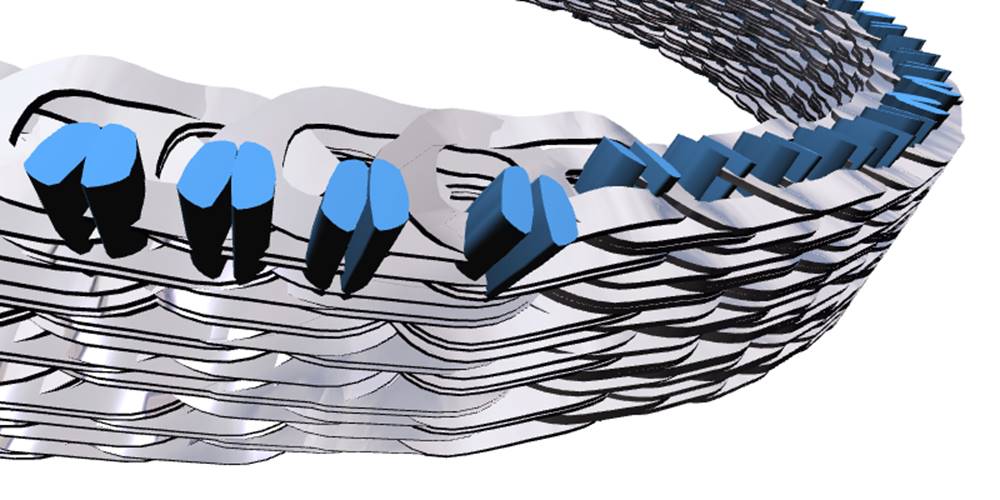
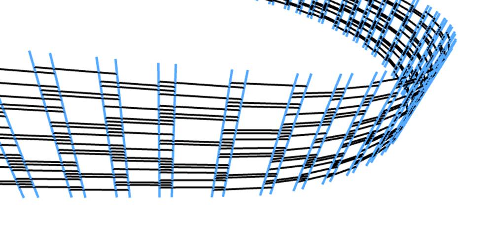
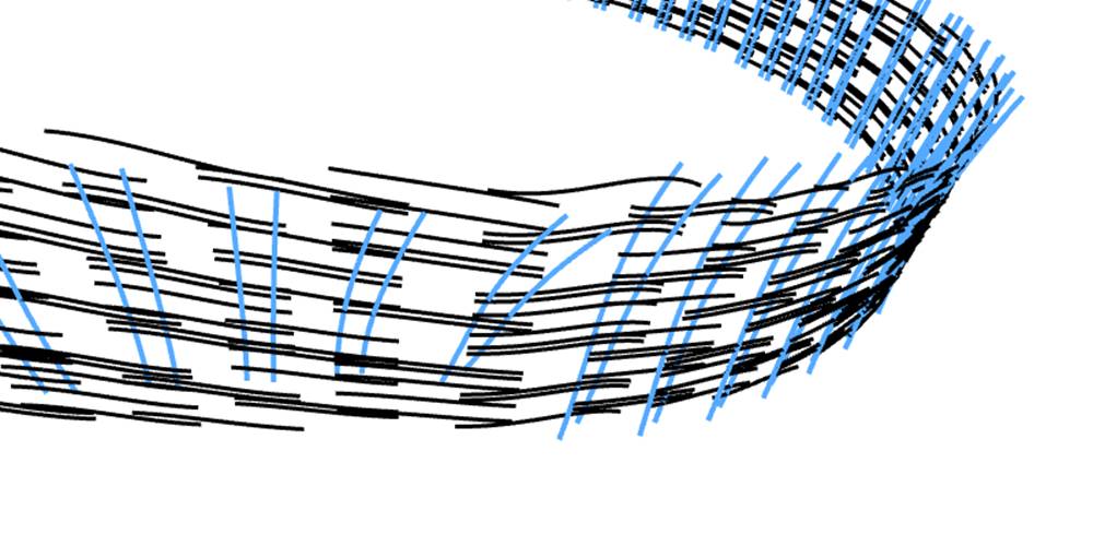
Fig. 8. Deformed CVT chain
6.1. Examples of deformed strip visualization
This subsection presents a number of images visualizing a strip deformed in different ways. Figure 8 shows part of CVT chain in a deformed state computed as a result of a simulation.
Figure 9 presents images of a separate strip in certain specific deformed states; the purpose is to show that the strip looks naturally for any possible deformable state. Green translucent shape represents the undeformed strip. Gray reflective shape represents the deformed strip. Subfigures (a)–(e) show rigid motion and deformations of compression, bending, and torsion separately; subfigure (f) shows an example of deformed state in the general case — all kind of deformations and rigid motion are present.
|
|
|
|
(a) rigid |
(b) compression |
|
|
|
|
(c) torsion |
(d) bending 1 |
|
|
|
|
(e) bending 2 |
(f) all |
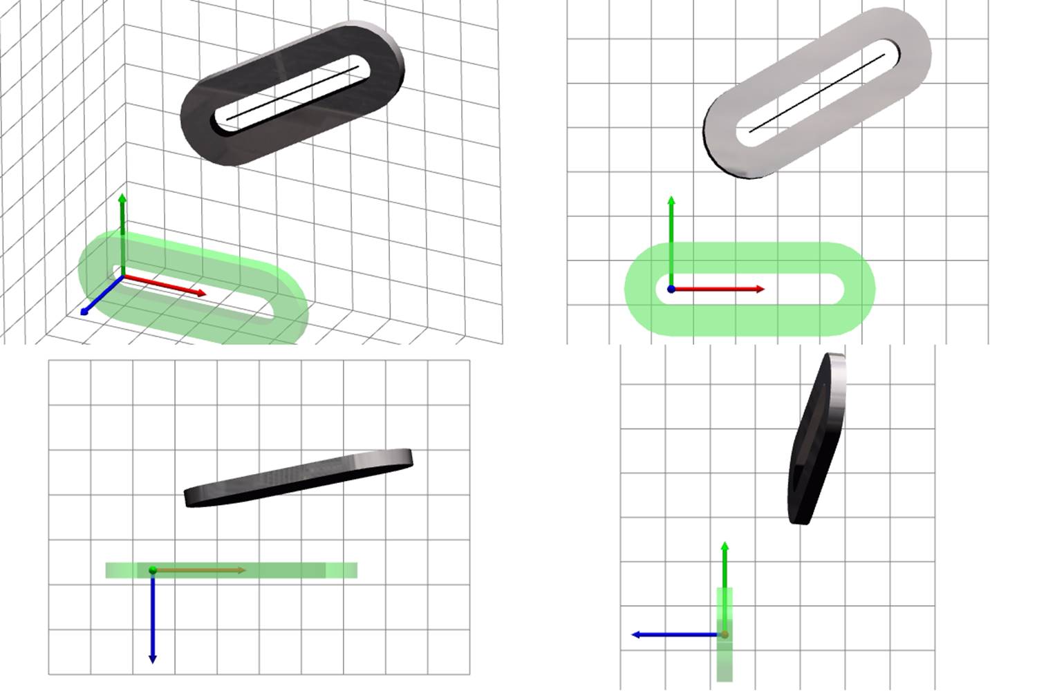
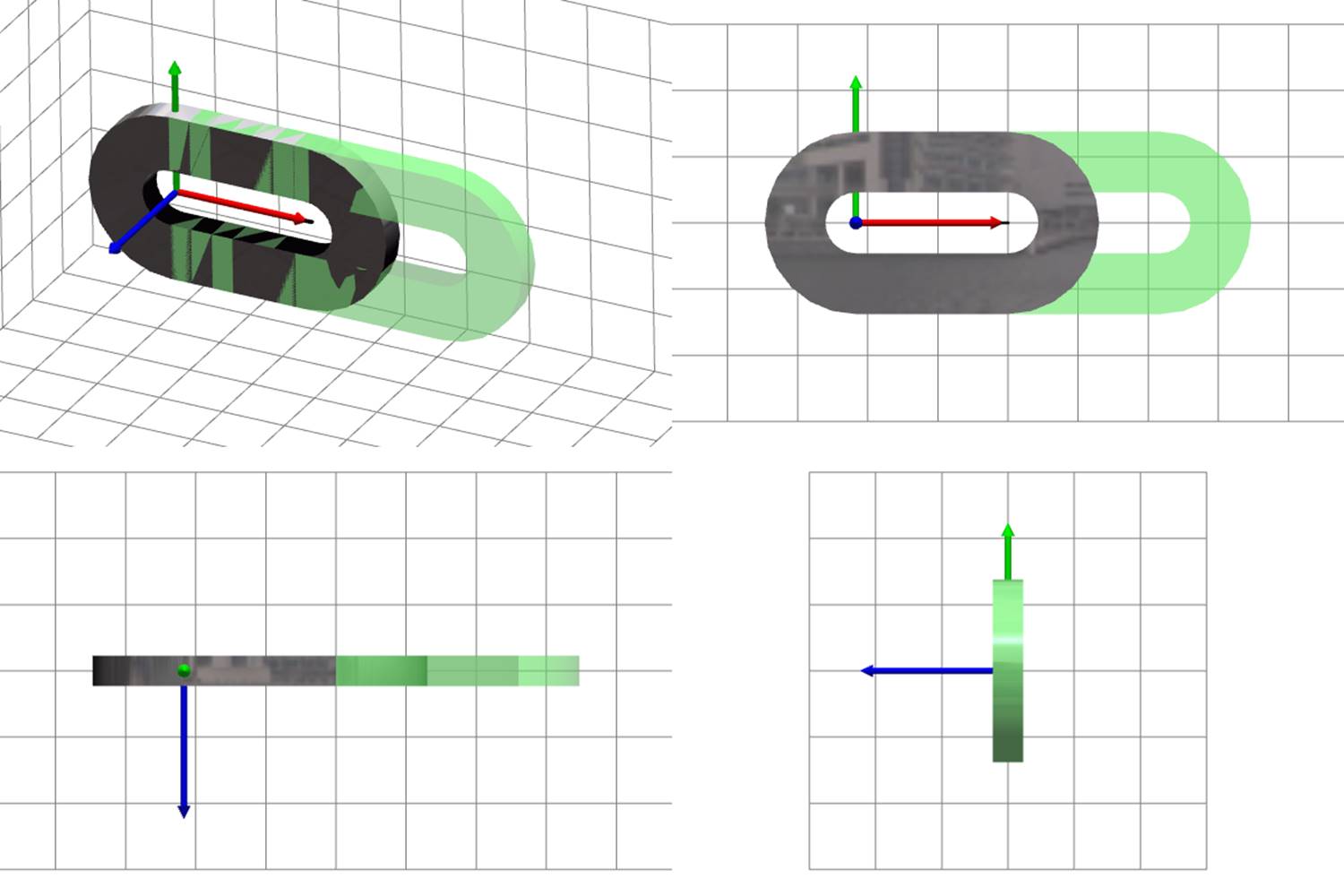
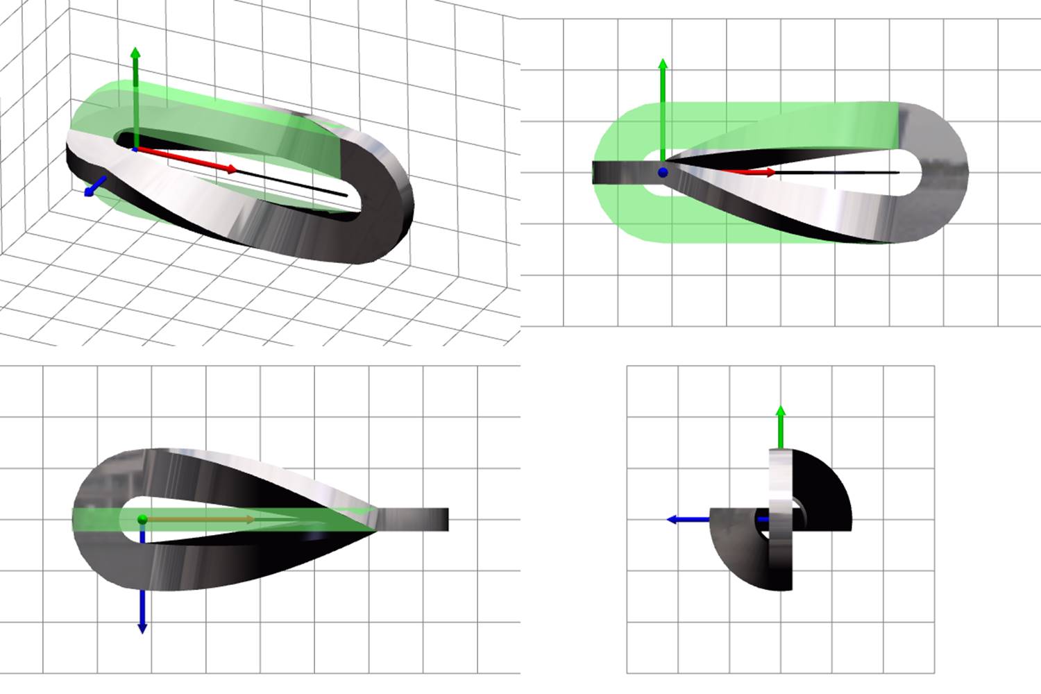
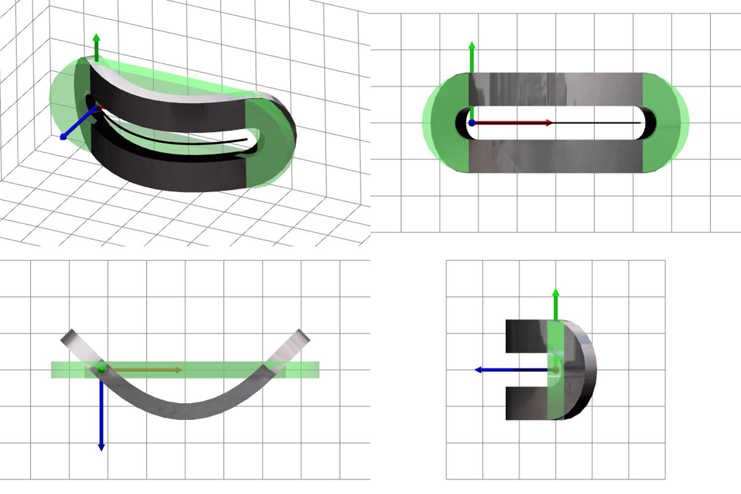
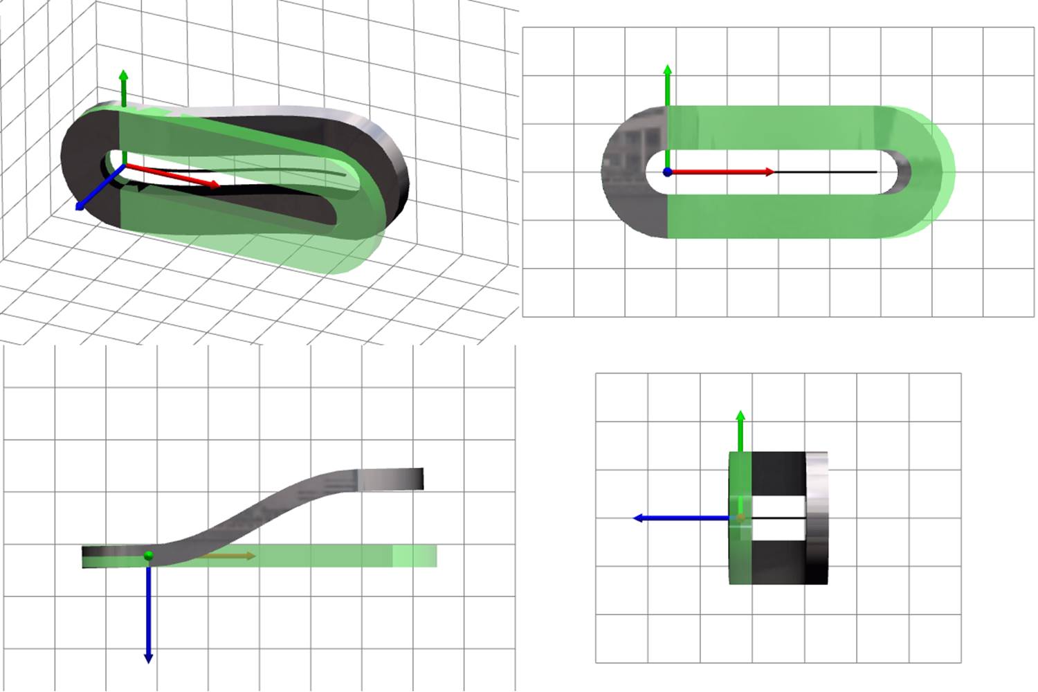
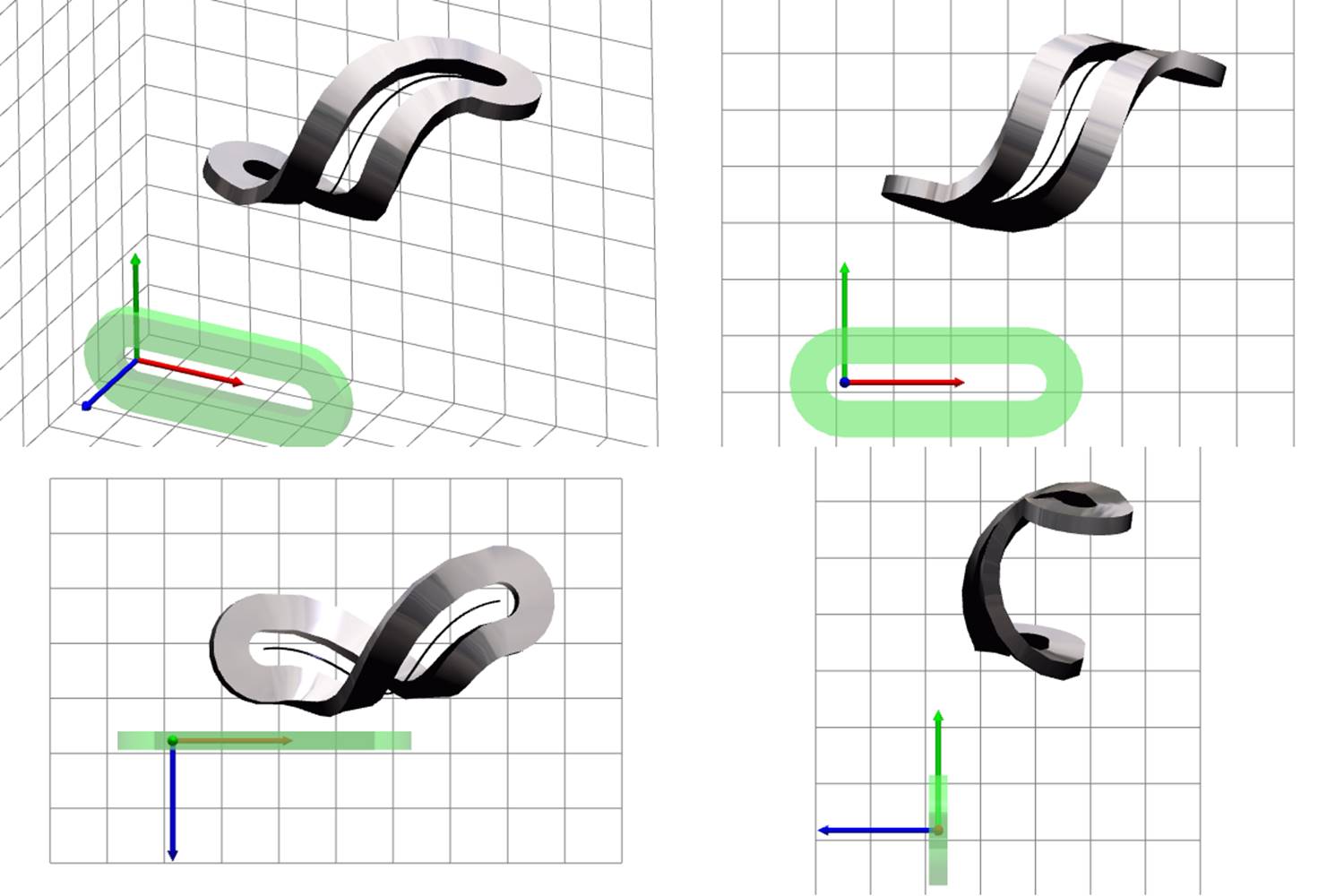
Fig. 9. Examples of visualization of deformed strip
|
#version 120 |
7. Conclusions
The paper proposes a definition of kinematics of deformable strip for use in the visualization of its deformed state. It is assumed that the deformed state is obtained without the consideration of large deformations. However, to see the deformed state with the naked eye, it is necessary to zoom the deformations. To make the zoomed deformed state look natural, non-linear kinematic relations have been considered. The constructed kinematics intentionally, for the sake of visualization simplicity, differs from what the non-linear theory of elastic rods [22] would give.
End parts of the strip are considered separately from the middle part because they do not deform and remain rigid. The rotations of these parts match the rotations of strip cross-sections at corresponding ends of the middle part.
The vertex shader implementing the developed kinematics relations for the deformable strip has been presented, and its complete source code is listed in the paper.
Examples of visualization are given to prove plausibility of the proposed kinematic relations.
Acknowledgements
Authors are thankful to the Russian Foundation for Basic Research for the support of this investigation carried out in the framework of grants No. 13-07-12077 and 14-07-00515.
References
[1] Legacy opengl. https://www.opengl.org/wiki/Legacy_OpenGL. [Online; accessed 05-02-2016].
[2] Nikolay Shabrov, Yuri Ispolov, and Stepan Orlov. Simulations of continuously variable transmission dynamics. ZAMM Zeitschrift f¨ur angewandte Mathematik und Mechanik. 94 (11):917–922, 11 2014.
[3] James F. Blinn. Simulation of wrinkled surfaces. SIGGRAPH Comput. Graph. 12(3):286–292, August 1978.
[4] Stanislav Klimenko, Lialia Nikitina, and Igor Nikitin. Real-Time Simulation of Flexible Materials in Avango Virtual Environment Framework. In Eurographics 2003 - Slides and Videos. Eurographics Association, 2003.
[5] Joachim Georgii and R¨udiger Westermann. Interactive simulation and rendering of heterogeneous deformable bodies. In Proceedings of Vision, Modeling and Visualization, pages 383–390, 2005.
[6] Cristian Luciano, Pat P. Banerjee, and Silvio H. R. Rizzi. GPU-based elastic-object deformation for enhancement of existing haptic applications. In CASE, pages 146–151. IEEE, 2007.
[7] Henry Sch¨afer, Benjamin Keinert, Matthias Nießner, Christoph Buchenau, Michael Guthe, and Marc Stamminger. Real-time deformation of subdivision surfaces from object collisions. In Proceedings of the 6th High-Performance Graphics Conference. EG, 2014.
[8] J. P. Lewis, Matt Cordner, and Nickson Fong. Pose space deformation: A unified approach to shape interpolation and skeleton-driven deformation. In Proceedings of the 27th Annual Conference on Computer Graphics and Interactive Techniques, SIGGRAPH ’00, pages 165–172, New York, NY, USA, 2000. ACM Press/Addison-Wesley Publishing Co.
[9] Doug L. James and Christopher D. Twigg. Skinning mesh animations. In ACM SIGGRAPH 2005 Papers, SIGGRAPH ’05, pages 399–407, New York, NY, USA, 2005. ACM.
[10] Eric Landreneau and Scott Schaefer. Poisson-Based Weight Reduction of Animated Meshes. Computer Graphics Forum, 2010.
[11] L. Kavan, P.-P. Sloan, and C. O Sullivan. Fast and Efficient Skinning of Animated Meshes. Computer Graphics Forum, 2010.
[12] Songrun Liu, Alec Jacobson, and Yotam Gingold. Skinning cubic b´Ezier splines and catmull-clark subdivision surfaces. ACM Trans. Graph., 33(6):190:1–190:9, November 2014.
[13] Carlos D. Correa and Deborah Silver. Programmable shaders for deformation rendering. In Proceedings of the 22Nd ACM SIGGRAPH/EUROGRAPHICS Symposium on Graphics Hardware, GH ’07, pages 89–96, Aire-la-Ville, Switzerland, Switzerland, 2007. Eurographics Association.
[14] John Isidoro and Drew Card. Animated Grass with Pixel and Vertex Shaders, pages 334–336. Wordware Publishing, Inc., Plano, Texas, 2002.
[15] K´evin Boulanger, Sumanta N. Pattanaik, and Kadi Bouatouch. Rendering Grass in Real-Time with Dynamic Light Sources and Shadows. Research Report PI 1809, 2006.
[16] Nico Galoppo, Miguel A. Otaduy, Paul Mecklenburg, Markus Gross, and Ming C. Lin. Dynamic deformation textures: GPU-accelerated simulation of deformable models in contact. 2007.
[17] Antoine Lambert, David Auber, and Guy Melan¸con. Living flows: Enhanced exploration of edge-bundled graphs based on gpu-intensive edge rendering. In Ebad Banissi, Stefan Bertschi, Remo Aslak Burkhard, John Counsell, Mohammad Dastbaz, Martin J. Eppler, Camilla Forsell, Georges G. Grinstein, Jimmy Johansson, Mikael Jern, Farzad Khosrowshahi, Francis T. Marchese, Carsten Maple, Richard Laing, Urska Cvek, Marjan Trutschl, Muhammad Sarfraz, Liz J. Stuart, Anna Ursyn, and Theodor G. Wyeld, editors, IV, pages 523–530. IEEE Computer Society, 2010.
[18] P. B´ezier. How Renault uses numerical control for car body design and tooling. In Society of Automotive Engineers Congress, 1968.
[19] E. Catmull and R. Rom. A class of local interpolating splines. Computer aided geometric design. Academic Press., pages 317–326, 1974.
[20] Philip Rideout. Path instancing. http://prideout.net/blog/?p=56, 2010.
[21] A. I. Lur'e. Nelinejnaja teorija uprugosti [Nonlinear theory of elasticity]. Nauka, Moscow, 1980
[22] V. V. Eliseev. Mehanika deformiruemogo tvjordogo tela [Mechanics of deformable solids]. Publishing house SPbPU, St. Petersburg, 2006.
[23] The opengl shading language, version 1.20. https://www.opengl.org/registry/doc/GLSLangSpec.Full.1.20.8.pdf. [Online; accessed 05-02-2016].
ВЕРШИННЫЙ ШЕЙДЕР ДЛЯ ВИЗУАЛИЗАЦИИ ДЕФОРМИРУЕМОЙ ПЛАСТИНЫ
С.Г. Орлов*, Н.Н. Шабров
Санкт-Петербургский политехнический университет Петра Великого, Кафедра компьютерных технологий в машиностроении
*Контактный автор: E-mail: majorsteve@mail.ru, телефон: +7 911 923 2705, Fax: +7 812 552 7770
Аннотация
Работа посвящена разработке вершинного шейдера для визуализации деформируемой пластины. Предложена аппроксимация геометрии пластины в деформированном состоянии, при этом учтена необходимость визуализации преувеличенных деформаций. Существенно, что деформированное состояние, подлежащее преувеличению и визуализации, соответствует решению задачи, в которой деформации считаются малыми. В этом случае преувеличенно деформированное состояние должно быть аккуратно определено, чтобы оно выглядело естественно. В работе также уделено внимание аппроксимации геометрии на концах пластины, где деформации отсутствуют. Приведён исходный код вершинного шейдера.
Ключевые слова: визуализация деформируемого тела, кинематика деформируемой пластины, преувеличенные деформации, вершинный шейдер, GLSL.