A SOLUTION TO A MULTIDIMENSIONAL DYNAMIC DATA ANALYSIS PROBLEM BY THE VISUALIZATION METHOD
D.D. Popov1, I.E. Milman1, V.V. Pilyugin1, A.A. Pasko2
1National Research Nuclear University MEPhI (Moscow Engineering Physics Institute), Moscow, Russian Federation
2National Centre for Computer Animation, Bournemouth University, Bournemouth, United Kingdom
dpopovmephi@gmail.com, igalush@gmail.com, VVPilyugin@mephi.ru, apasko@bournemouth.ac.uk
Contents
2.1. Description of the dynamic geometrical processes
2.2. Formal description of the problem solution process by the visualization method
2.3. Visualization of source data
3. Description of the solution algorithm
4. Description of the application program
4.1. Options of the application program
4.2. Examples of use of the application program
Abstract
The article describes a solution of a data analysis problem. Data to be analyzed represent changes in a given set of multidimensional objects with time. We propose to apply the visualization method to solve this problem. A formalization of the method is presented with a mathematical description of each stage of the source data visualization.
A developed interactive visualization application program is described. It is based on the models of the theoretical part of the article.
We emphasize the efficiency of the visualization method. It allows one to make a judgment on the formation of bunches or clusters of objects formalized in the form of n-tuples of real numbers and to find the objects seeking to be in a cluster or a bunch. Additionally, examples of use of the developed program for searching for invariants in changing the source data are provided.
Keywords: multidimensional analysis, dynamic data analysis, visual analysis, multidimensional visual analysis.
1. Introduction
There is an urgent problem of processing and analysis of multidimensional data in the modern world. For its solution there are developed many different methods and means, both automatic and interactive. Visual methods occupy a special place among data analysis methods.
However, a careful study of the literature devoted to the description of particular applications that use visual methods suggests that interactive systems working with multi-dimensional data are often valued less than systems that depict results of application of the Data Analysis methods. For example, there are such systems as the system of situational notification AdAware [1], the system of visual analysis in aircraft design problems [2], the visual analysis of textual information VxInsight, software package SAS Visual Analytics [3] designed for processing and analyzing large volumes of financial and economic information. All these systems are of an industrial nature are commercial, the systems provide the user with a great number of interfaces and data visualization capabilities. However, at the same time, all these systems are adjusted to the internal processing of these multidimensional data and presentation of these data to the user in a convenient way, without giving to the user either a possibility to work directly with the cloud data or to work with multivariate visual representation of the data [4, 7].
Theoretical generalizations of a solution of a problem of a source data analysis using the visualization method that was based on scientific data are considered in [5]. This method can be divided into the two following stages that in general can be repeated:
- visualization of source data;
and
- analysis of images that is followed by formulation of judgments about source data.
The original analysis algorithm of multidimensional geometric data based on this method is presented in [6]. A visualization application program based on this algorithm was developed. This application’s main feature is the possibility to work with multidimensional source data directly. The analyst purposeful manipulate directly with the source data and perform visual analysis of the results without making any original numerical processing of the source data. The paper shows that the application program can effectively solve a problem of multidimensional static source data analysis.
However, in practice we have to deal very often with multidimensional dynamic source data: monthly or annual organizations’ reports, elementary particles’ properties in different time periods, etc. These data contain information about the progress of these objects with time. The analyst wants to make a judgment about this progress, i.e., a judgment about the multidimensional dynamic source data. This article discusses developed mathematical models of dynamic multidimensional source data and the interactive application program that allows the analyst to analyze the data by the visualization method.
2. Formulation of the problem
Dynamic source data are values of some quantitative
characteristics of these objects, which can change during the time. Each object
can be denoted by an n‑tuple of real numbers in a fixed moment in time.
We will consider the n-tuples of real numbers as points in a multidimensional
Euclidean space ![]() with
a defined distance. Thus we assign a multidimensional dynamic data analysis
problem by the visualization method with a geometric interpretation, i.e. the
task of the analysis of change in the relative position of the points in the
space
with
a defined distance. Thus we assign a multidimensional dynamic data analysis
problem by the visualization method with a geometric interpretation, i.e. the
task of the analysis of change in the relative position of the points in the
space ![]() .
.
Subsets of points representing clots and clusters can be allocated in this space, these subsets are described in [4]:
A cluster - a subset within a given point set, where the pairwise distance does not exceed the pre-defined d value and the distance between cluster points and other points is not less than the pre-defined d value.
A bunch - a subset of points with most distances between points not exceeding the preset d value.
In a particular way subsets may consist of a single point, in [4] the following points classification is given:
A remote (single) point - a point distant from all other points of the initial set for more than the preset d value.
Quasi-remote (quasi-single) point - a point that is not remote but at the same time is not included in a bunch or a cluster at the given grouping.
Isolation of clots and quasi-remote points performs by a man in the process of solving analysis problem.
Note that remote and quasi-remote points are special cases of clusters and clots respectively.
The values of the coordinates of points can change over time. Points can form clots and clusters or join them over time and vice versa.
The main purpose of this work is the solution of the
analysis problem of changes of the mutual arrangement of the assigned set of
the points in space ![]() by
the visualization method. In achieving this purpose, a solution of a
multidimensional dynamic data analysis problem by the visualization method will
be found.
by
the visualization method. In achieving this purpose, a solution of a
multidimensional dynamic data analysis problem by the visualization method will
be found.
The solving of the problem can be divided into the following stages:
· Making a mathematical description of the objects analyzed.
· Development of an algorithm for a solution of a multidimensional dynamic data analysis problem by the visualization method.
· Writing an application to solve the analysis problem.
Let us introduce the following notions that will be used to describe the subsequent material.
A Geometric Process is a set of points in space, coordinates of which are time-dependent.
We call a spatial process the variable spatial scene depending on the time. In other words, a spatial process is a dynamic spatial scene. Detailed description of the scene will be given below (paragraph Mapping).
2.1. Description of the dynamic geometrical processes
The initial object of the analysis is a set of n-dimensional
points ![]() .
Coordinates of the points are given in several time instants:
.
Coordinates of the points are given in several time instants: ![]() .
.
A point has n coordinates:
![]()
the distance for each pair of point equals:
![]()
We have the discrete geometrical process in the
beginning: ![]() , it
consists of discrete processes
, it
consists of discrete processes ![]() –
dynamic n-dimensional points, which are given by
–
dynamic n-dimensional points, which are given by ![]() –
their dynamic coordinates.
–
their dynamic coordinates.
The process ![]() is a
chronological geometrical description of states of the items involved. However,
the items change continuously. We use an interpolation to describe the
continually changing items.
is a
chronological geometrical description of states of the items involved. However,
the items change continuously. We use an interpolation to describe the
continually changing items.
Process ![]() were
interpolated using piecewise linear interpolation technique. In this case, the
desired interpolation function for time-dependent coordinates of points
were
interpolated using piecewise linear interpolation technique. In this case, the
desired interpolation function for time-dependent coordinates of points ![]() is
binomial
is
binomial ![]() in
closed interval
in
closed interval ![]() ,
, ![]() . For
a value
. For
a value ![]() ,
, ![]()
![]() is
given from the equation:
is
given from the equation:
![]()
The result of the interpolation ![]() is a geometrical
continuous process. Then
is a geometrical
continuous process. Then ![]() is a
temporal section,
is a
temporal section, ![]() belongs
to the domain of
belongs
to the domain of ![]() .
.
![]() can be discretize using temporal
sections. The discrete geometrical process is the collection of temporal
sections for selected
can be discretize using temporal
sections. The discrete geometrical process is the collection of temporal
sections for selected ![]() . So
. So ![]() is
is ![]() temporal
sections of the
temporal
sections of the ![]() process.
process.
2.2. Formal description of the problem solution process by the visualization method
We use the visualization method [5] to solve this problem. The method is based on the sequential solution (generally multiple) of the two tasks presented below:
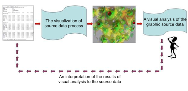
Fig. 1. The visualization method
The analyst specifies visualization parameters and obtains static or animated images (i.e chronological frames) until he/she is able to make his/her own judgment on changes in the relative position of points with time. Thus a solution of a multidimensional dynamic data analysis problem by the visualization method is interactive.
A visualization application program should provide an interactive user interface. The analyst should have an opportunity to influence a spatial scene and obtained images. This makes solving of the problem much more efficient. Thus a solution of a multidimensional dynamic data analysis problem by the visualization method is iterative and interactive.
The visualization process of the source data will be reviewed below.
2.3. Visualization of source data
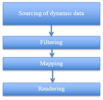
Fig. 2. Source data visualization
Sourcing of dynamic data
The discrete geometric process ![]() is specified in this
step. This process
is specified in this
step. This process ![]() be
visualized later on.
be
visualized later on.
Filtering
In this step, the source data are preprocessed.
The initial discrete process ![]() is
interpolated using piecewise linear interpolation technique as described
earlier. The result of filtering is an obtained continuous process
is
interpolated using piecewise linear interpolation technique as described
earlier. The result of filtering is an obtained continuous process ![]() .
.
Mapping
The Analyst selects a 3-dimensional subspace of the
n-dimensional space that will be used to create a continuous spatial processes.![]() are
numbers of basis vectors of the original n-dimensional space. They form the
basis of the subspace.
are
numbers of basis vectors of the original n-dimensional space. They form the
basis of the subspace.
The initial set of points is projected onto the selected subspace.
![]() is
the set of projections,
is
the set of projections, ![]() .
.
After that, the analyst selects the radius of spheres ![]() that
are associated with the obtained 3-dimensional points, their color
that
are associated with the obtained 3-dimensional points, their color ![]() and the radius of
cylinders
and the radius of
cylinders ![]() that
connect the spheres with each other. The distance between the connected spheres
is less than the assigned d. associating with points the distance between which
is less than the assigned d.
that
connect the spheres with each other. The distance between the connected spheres
is less than the assigned d. associating with points the distance between which
is less than the assigned d.
Spatial scene ![]() corresponds to the obtained continuous
geometric process
corresponds to the obtained continuous
geometric process ![]() , which is a result of interpolation of
the source discrete geometric process
, which is a result of interpolation of
the source discrete geometric process ![]() .
. ![]() is the description of
the scene geometry and
is the description of
the scene geometry and ![]() is the description of the optical
parameters of the scene. The scene is a continuous spatial process:
is the description of the optical
parameters of the scene. The scene is a continuous spatial process:
![]() .
.
Then at each fixed ![]() ,
, ![]() will
correspond to
will
correspond to ![]() ,
, ![]() . Let
us define
. Let
us define![]() .
.
![]()
where ![]() is a
sphere of radius
is a
sphere of radius ![]() centered
at the point
centered
at the point ![]() ,
, ![]() is a
cylinder of radius
is a
cylinder of radius![]() that
connects two spheres,
that
connects two spheres, ![]() .
.
![]()
where ![]() is a
color of the spheres,
is a
color of the spheres, ![]() are
colors of the cylinders.
are
colors of the cylinders.
![]() is a
color and opacity of the
is a
color and opacity of the ![]() -th cylinder that connects spheres
associated with points
-th cylinder that connects spheres
associated with points ![]() . The
color is defined in RGB, the opacity is defined in RGB as well:
. The
color is defined in RGB, the opacity is defined in RGB as well:
![]()
![]()
![]()
![]()
![]()
![]()
where ![]() means that the cylinder is completely
transparent,
means that the cylinder is completely
transparent, ![]() % – means that the cylinder is completely
opaque.
% – means that the cylinder is completely
opaque.
Spatial discrete process space ![]() can
be created from this continuous process as described above for the geometric
continuous process
can
be created from this continuous process as described above for the geometric
continuous process ![]() .
.
For example, this option may be necessary if the analyst is interested only in the key moments which show a clot or a cluster formation.
Rendering
The projection image ![]() is the
result of a scene’s
is the
result of a scene’s ![]() rendering. A scene is a process:
rendering. A scene is a process: ![]() . We
have the scene and, therefore, the projection image for each time t. Let us
enter one more process
. We
have the scene and, therefore, the projection image for each time t. Let us
enter one more process ![]() .
.
![]()
where ![]() is a
set of visualization attributes.
is a
set of visualization attributes.
Visualization attributes are a camera ![]() ,
light, physical characteristics of the scene environment, size of an obtained
image, etc. They can be either static or dynamic.
,
light, physical characteristics of the scene environment, size of an obtained
image, etc. They can be either static or dynamic.
By camera we mean the point of view which fix the scene ![]() .
. ![]() where
where
![]() is
the camera position,
is
the camera position, ![]() is
the focus and
is
the focus and ![]() is the camera angle.
is the camera angle.
The sequence of frames ![]() is
the result of discrete spatial process’s
is
the result of discrete spatial process’s ![]() rendering.
Frames
rendering.
Frames ![]() can
be used as key frames for the construction of the animation.
can
be used as key frames for the construction of the animation.
3. Description of the solution algorithm
The algorithm for solving the problem consists of the following steps:
- dynamic source data input;
- their interpolation and obtaining of a continuous geometric process;
- setting d and static scene parameters: the spheres’ radii, the cylinders’ radii, the projection subspace, the spheres’ color;
- construction of a continuous geometric process that uses predefined static parameters;
- construction of temporary sections of continuous spatial process, or its sampling;
- setting camera and other visualization attributes for rendering;
- construction of projection images of the spatial discrete process;
- further preservation of projection images in the sections gallery or a creation of an animated film.
In case if the obtained projection images are not enough, and the analyst cannot make judgment about interesting in his opinion data, the algorithm provides returns to the scene setting stage and to the stage of setting visualization attributes.
The algorithm described above is shown below in Figure 3.
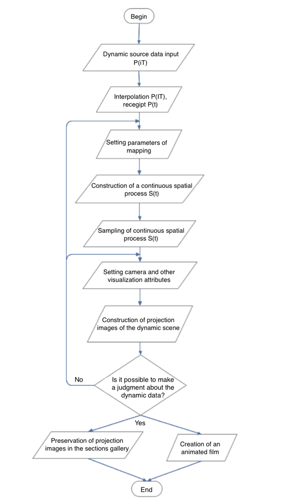
Fig. 3. Solution algorithm
4. Description of the application program
We developed an interactive visualization application program to solve the problem of the analysis of changes in the relative position of points. The application program is based on the algorithm shown above.
4.1. Options of the application program
The application program gives the analyst the following options:
- Dynamic source data input from a special text file.
- Piecewise-linear interpolation of the discrete geometric process.
- Construction of a dynamic scene associated with geometric continuous process.
- Setting of visualization attributes.
- Construction of the projection image of the spatial discrete process.
- Saving obtained projection images.
- Animation construction.
The developed application program provides user-friendly and interactive visual interface that allows the analyst to manipulate the rendered space scene.
We used 3ds Max® application program and its internal object-oriented programming language MAXScript.
4.2. Examples of use of the application program
The program was tested using the source data containing monthly reports of credit institutions.
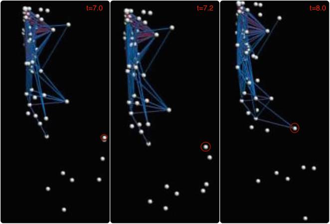
Fig. 4. Images from the "sections gallery" obtained for the credit institutions’ data.
The moment when the distant point joint the clot was
discovered as a result of the images (Fig. 4) analysis. The judgment that has
been made is that the point of the subset became the point of another subset
during the time ![]() .
.
After analyzing animation shown in Figure 5, we can make an interesting conclusion.
Fig. 5. The result of dynamic spatial process rendering
All sectors associated with the initial n-dimensional points are approximately located in one plane.
This observation enables us to make the following judgment.
The equation ![]() is
right for the projections of points' coordinates
is
right for the projections of points' coordinates ![]() on
the selected subspace
on
the selected subspace ![]() .
. ![]() are
constants.
are
constants.
Source data was calculated by the method of least squares, and the following equation of approximating plane was carried out:
![]()
In the examples above, numbers![]() correspond
to the coordinates which values reflect the following financial indicators of
credit institutions:
correspond
to the coordinates which values reflect the following financial indicators of
credit institutions:
- overdue debt in the loan portfolio;
- issued bonds and notes;
- net assets issued interbank loans.
Note that a similar approach, based on an approximation of the planes in the space of principal components used in [8,9].
5. Conclusion
In this paper, we have:
- presented a mathematical description of discrete and continuous processes;
- developed an algorithm of solution of a multidimensional dynamic data analysis problem by the visualization method;
- presented an interactive application program based on the developed algorithm;
- tested application program using the dynamic monthly performance financial data;
- made judgments about these data.
The interactive user interface allows a user to find the time when points form clusters and clumps and vice versa. The developed application program provides user-friendly interactive visual interface that allows the analyst to manipulate the rendered space scene.
We can say that the developed application program performs dynamic animated visualization of multidimensional source data. This application program automatically creates a description of the key spatial scenes, which are animated then.
In addition, the user is given an opportunity to cut out an interesting in his opinion part of the process. He can control the speed of the process’ flow in the resulting animation. These options are available interactive.
The nature of the dynamic source data may require another type of the data interpolation, thus we plan to make it possible to choose an another interpolation technique in the next version of the application program. Another direction of the research is geometric and spatial processes of operator variable.
References
1. Livnat Y., Agutter J., Moon S., Foresti S. Visual correlation for situational awareness. IEEE Symposium on Information Visualization. pp. 95-102, 2005.
2. Mavris D., Pinon O., Fullmer D.Jr. Systems design and modeling: A visual analytics approach. 27th Congress of International Council of the Aeronautical Sciences ICAS, 2010.
3. SAS the power to know. URL: http://www.sas.com/en_us/home.html. [Access date: 26 1 2016].
4. Maslennikov O.P., Milman I.E., Safiullin A.E., Bondarev A.E., Nizametdinov Sh.U., Pilyugin V.V. Razrabotka sistemy interaktivnogo vizualnogo analiza mnogomernykh dannykh [Development of a system for analyzing multidimensional data]. Scientific visualization. V.6, no. 4, p. 30-49, 2014. (in Russian)
5. Pilyugin V., Malikova E., Pasko A., Adzhiev V. Nauchnaja vizualizacija kak metod analiza nauchnyh dannyh [Scientific visualization as method of scientific data analysis]. Scientific Visualization. V. 4, no. 4, pp. 56-70, 2012 (in Russian)
6. Milman I.E., Pakhomov A.P., Pilyugin V.V., Pisarchik E.E., Stepanov A.A., Beketnova Yu.M., Denisenko A.S., Fomin Ya.A. Data analysis of credit organizations by means of interactive visual analysis of multidimensional data. Scientific Visualization. 2015. V. 7, no. 1, pp. 45 – 64
7. Maslennikov O.P., Milman I.E., Safiullin A.E., Bondarev A.E., Nizametdinov Sh.U., Pilyugin V.V. Interaktivny vizualny analiz mnogomernykh dannykh [Interactive visual analysis of multidimensional data]// GraphiKon'2014: 24th International conference on computer graphics and vision: Rostov-on-Don, the SFU Academy of architecture and arts, Conference materials. - p. 51-54 (in Russian)
8. Bondarev A.E, Galaktionov V.A. Parametric Optimizing Analysis of Unsteady Structures and Visualization of Multidimensional Data. International Journal of Modeling, Simulation and Scientific Computing. 2013. V.04. N supp01. 13 p. DOI 10.1142/S1793962313410043.
9. Bondarev A.E. Analiz mnogomernyh dannyh v zadachah vychislitel'noj gazovoj dinamiki [Multidimensional data analysis in cfd problems]. Scientific visualization. Vol. 6. No. 5. Pp. 61-68. 2014.