METHOD FOR DATA STATISTICAL COMPARISON VISUALIZATION
A.V. Maksimushkina1, V.V. Smirnova2
1National Research Nuclear University MEPhI (Moscow Engineering Physics Institute)
2National research centre "Kurchatov Institute" Institute for high energy physics
AVMaksimushkina@mephi.ru, Vera.Smirnova@ihep.ru
Contents
2. Method and software for calculated and experimental data statistical comparison
3. Selection of neural network for effective approximation of the data
Abstract
Different methods for the calculated data analysis, the choice or comparison of the calculation models are used and their specific application depends on the tasks set. One of the new techniques that can be applied to such problems is the data statistical comparison method. This method is used for the nuclear reaction cross sections obtained using specialized calculation programs analysis.
Keywords: nuclear reaction cross-section, data analysis, visualization, neural network, approximation
1. Introduction
Preparation of data on nuclear reaction cross sections is an important task for the design and practical problems in the areas of nuclear technology. Obtaining these data in experiment is technically challenging and expensive procedure. That is why specialized computer codes and programs based on physical models of the complex processes that occur during the nuclei with protons or neutrons interaction are often used. Thus, the urgent tasks are as follows: verification of how well the model describes the experimental data, selection of the model or choice of the model parameters. There are many methods for comparison of experimental and /or calculated data [1], whose specific application depends on the tasks set.
Let us assume that there are two data sets of the same size, which are measured or calculated values of a random variable depending on another (nonrandom) variable. It is required to determine how compatible these two sets of data are. As compatibility of these sets we assume that for each value of the nonrandom variable both treated samples are taken from the same general population.
Most methods of data comparison are based on the calculation of a one-dimensional test statistics, allowing to estimate how much the compared data differ from each other. It is generally assumed that the possible distribution of the test statistics (for example, χ2 and Kolmogorov statistic) is known. To solve such problems, the method for statistical comparison of data can be used [2]. The method uses a two-dimensional test statistic. The possible distributions of the test statistics (calibrated and testing) are constructed by Monte Carlo. The degree of difference for the distributions constructed is determined due to testing two hypotheses:
· the main H0 hypothesis: the data sets being compared are compatible (both samples are taken from the same general population), against
· the alternative H1 hypothesis: compared data sets are incompatible (samples are taken from different populations).
Representation of the results of two data sets comparison as two-dimensional distributions (calibration and test) makes the possibility both to show the integral difference between data sets and to give a numerical estimate of this difference.
2. Method and software for calculated and experimental data statistical comparison
The statistical comparison of data method is an extension of
the histogram comparison method [3-5]. It uses statistical moments of the
distribution ![]() ("the
significance of difference"), where
("the
significance of difference"), where![]() is
the number of compared points in the compared data tables. This distribution
consists of M values. If both sets of data are obtained from the same
population, then the distribution is close to the standard normal distribution,
because each realization of
is
the number of compared points in the compared data tables. This distribution
consists of M values. If both sets of data are obtained from the same
population, then the distribution is close to the standard normal distribution,
because each realization of ![]() of
random value for each compared point i is a realization of the random
variable that obeys to law close to standard normal law.
of
random value for each compared point i is a realization of the random
variable that obeys to law close to standard normal law.
Thus, the two-dimensional value SRMS = (![]() , RMS) serves
as the distance between data sets, where
, RMS) serves
as the distance between data sets, where  is the mean value of the distribution of
"significances of difference" and
is the mean value of the distribution of
"significances of difference" and  is the standard deviation of this distribution.
To compare two sets of data, the significance of the difference in relevant measuring points is defined as follows:
 ,
,
where nik is the observed value at the measurement point i-th set of data k, σik is the corresponding standard deviation.
For each of the compared sets of data a number of similar data sets (clones) are created in accordance with the model under consideration. The value at each measurement point is generated according to the normal distribution. This allows one to create two sets of imitating models of two corresponding populations for data sets, which must be compare. In constructing the two-dimensional calibration distribution for the possible values of the test statistic in the frame of first imitating model of the population, a comparison is made of the data sets obtained during the construction of the sets of data like the first original set (i.e. the cloning). In constructing the test distribution of possible values of the two-dimensional test statistic, comparisons of datasets obtained by the cloning the first original data set are performed with the sets of data obtained by the cloning the second original data set. During each comparison the distribution of significances of difference is built in the respective measurement points, after that the average and the root mean square values are determined for the distribution obtained. These values are used to test the hypotheses about the compatibility of data sets.
To distinguish between the hypotheses in comparing the data sets the significance level criterion is defined, i.e. the probability to make a mistake of the first α type. For the two-dimensional distribution (S, RMS) after setting the significance level criterion the critical line for determining the power of a test is selected, relative to which there is a type II error. Then we calculate the test power of 1-β, where β is the probability of an error of the second kind. The probability of correct decisions that data sets are distinguishable is defined as [6]:
![]() .
.
The method of statistical comparison of data is realized in
the program [7] designed to analyze data and simulation models. The program is
written in the programming language C # [8] and has an intuitive clear
interface. The user needs to set the number of clones, the error of the first
type, and select the file with which the data will be compared. The results are
displayed in graphs and distributions ![]() and RMS (Figs. 1-2.), the probability that the
compared data do not belong to the same general population is also calculated.
and RMS (Figs. 1-2.), the probability that the
compared data do not belong to the same general population is also calculated.
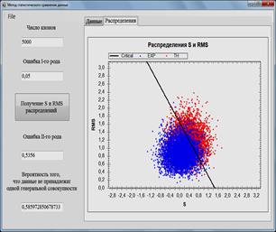
Fig. 1. Software for data analysis and simulation models. Comparison of the calculated and experimental data.
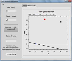
Fig. 2. Software for data analysis and simulation models. Comparison of the calculated data obtained by two models with experimental data.
3. Selection of neural network for effective approximation of the data
One way to get the evaluated data is an approximation of available experimental values. Neural networks can be used to approximate the experimental values. The efficiency and quality of such approximations are shown in [9], where several structures of neural networks are discussed and the quality of the approximation is evaluated using consent factors. Alternatively, an analysis was performed by the method for statistical comparison of data for determining the structure of the neural network which provides the best match with the experimental data. The data for which an approximation was performed using neural networks are cross sections of the 209Bi (p,4n)206Po reaction, which were taken from the EXFOR experimental data library [10]. Fig. 3 presents data on the cross sections in the mbarn range, depending on the energy in MeV.
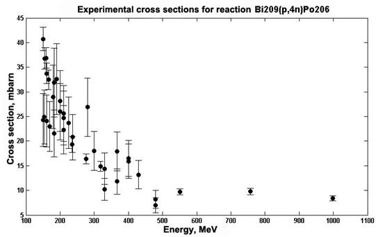
Fig.3. The cross sections of reaction 209Bi (p,4n)206Po depending on the energy
Four neural networks (Newfit, Newpr, RBF, GRNN) [11-14] were selected which are integrated in MatLab [13, 14]. The implementation was carried out in the system MatLab which allows one to create and describe in detail the neural network by varying the various parameters of the network and the use of different activation functions.
Network diagrams, which were used for the calculations are presented in Table 1.
For each network configuration an approximation has been done of the selected data in order to identify the network that best describes the behavior of the data.
Further, two-dimensional distribution values of ![]() and the RMS were
obtained for the initial data set for each set of calculated values obtained
with the four configurations of neural network (Newfit, Newpr, RBF, GRNN). The
distributions are shown in Fig. 4.
and the RMS were
obtained for the initial data set for each set of calculated values obtained
with the four configurations of neural network (Newfit, Newpr, RBF, GRNN). The
distributions are shown in Fig. 4.
Table 1. Neural Network diagrams
|
Neural Network |
Description |
|
Newfit
|
You can use any differentiable activation function as activation functions, for example, the hyperbolic tangent, sigmoid function. You can use any function as a learning function on the basis of the back-propagation algorithm. The first layer consists of 50 neuron hyperbolic tangent activation function, the second layer of one neuron with linear activation function. |
|
Newpr (pattern recognition network)
|
Any differentiable activation function can be used as activation functions (hyperbolic tangent, sigmoid function). You can use any function as a learning function on the basis of back-propagation algorithm. The first layer consists of 100 neurons with the hyperbolic tangent activation function, the second layer of one neuron with the same activation function. |
|
RBF (radial basis)
|
The two-layer network with no feedback contains a hidden layer of radially symmetric hidden neurons. The activation function is the Gaussian function. |
|
GRNN (General Regression Neural Network)
|
The first intermediate layer consists of a network GRNN radial elements. The second intermediate layer (linear) includes elements which serve to estimate the weighted average. The activation function is the Gaussian function. |
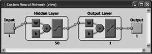

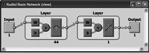
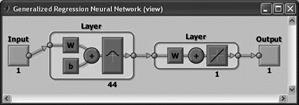
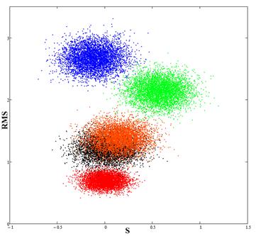
Fig.4. The red spot (calibration) corresponds to experimental data; the blue spot is the result of the comparison of data for Newfit and experimental data; the green spot is the result of the comparison of data for Newpr and experimental data; black and orange spots (almost overlapping) is the result of the comparison of RBF and GRNN results with the experimental data.
Thus, the data obtained using RBF and GRNN networks, are nearest to the experimental data.
Also the quality of the approximation calculations was evaluated using consent factors [15] (Table 2).
Table 2. Description of consent factors
|
F |
|
Evaluation of the integrated proximity to experiment for widely differing data. |
|
D |
|
It reflects the acceptable degree of compensation of small values by some large values of other terms. The higher the value, the greater the possible compensation. |
|
H |
|
|
|
R |
|
Evaluation of the relative proximity of the integrated data. |
N is the total number of data points, ![]() - experimental values of
cross sections,
- experimental values of
cross sections, ![]() -
calculated values of cross sections,
-
calculated values of cross sections, ![]() - the error of experimental cross sections.
- the error of experimental cross sections.
The results of calculation of consent factors are presented in Table 3.
Table 3. Results of calculation factors
|
|
F |
D |
R |
H |
|
Newfit |
1.854 |
0.226 |
1.02 |
2.484 |
|
Newpr |
1.237 |
0.168 |
0.973 |
1.99 |
|
RBF |
1.114 |
0.065 |
1.006 |
0.72 |
|
GRNN |
1.135 |
0.09 |
1.009 |
0.99 |
As can be seen from Table 3, the approximations obtained by RBF and GRNN have the best match with the experimental data, which is consistent with the results obtained using the method of statistical comparison.
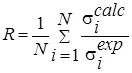
Also, an analysis is made of the data obtained using the RBF network for cross sections of the 209Bi (n, 3n) 207Bi reaction. The data are compared with the experimental values and the data taken from the FENDL library [16] (Fig. 5).
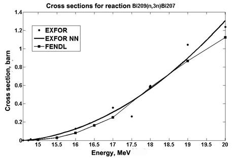
Fig.5. Cross section data for reaction 209Bi (n, 3n)207Bi
The results of the construction of the distribution are presented in Fig. 6.
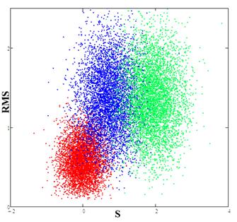
Fig.6. Red spot (calibration) corresponds to the experimental data; the blue spot is the result of the comparison data for the RBF network and the experimental data, the green spot is the result of the comparison of data from the FENDL library with experimental data.
From Fig. 6 it is seen that the distribution obtained for the neural RBF network lies closer to the calibration and hence the model constructed using the neural network provides a better description of the experimental data. Thus, to obtain more accurate calculations in which cross-section data are used for example as in [17,18], it is preferable to use the data obtained by the RBF network.
4. Choice of model parameters
Estimates of nuclear reaction cross sections were carried out in the ALICE / ASH program for different E0 parameters (parameters responsible for the pre-equilibrium emission of clusters) and PLD (parameter of levels density) [19]. An analysis was made in order to select the parameters in which the estimates are in better agreement with experimental values. Figs. 7-8 show the results of calculations for the natFe (p, x) 10Be reaction.
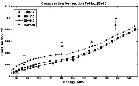
Fig. 7. Experimental and calculation cross sections for the natFe(p,x)10Be (PLD=12.7)reaction
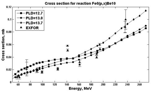
Fig. 8. Experimental and calculation cross sections for the natFe(p,x)10Be (E0=7.5) reaction
For all values of the parameters consent factors have been calculated (Table 4).
Table 4. Results of calculation of consent factors
|
|
F |
D |
R |
H |
|
E0=7.2, PLD=12.7 |
1.27 |
0.13 |
0.89 |
1.10 |
|
E0=7.5, PLD=12.7 |
1.22 |
0.16 |
1.05 |
2.11 |
|
E0=8.2, PLD=12.7 |
1.60 |
0.54 |
1.54 |
6.64 |
|
E0=7.5, PLD=13.0 |
1.23 |
0.19 |
1.09 |
2.19 |
|
E0=7.5, PLD=13.7 |
1.33 |
0.31 |
1.23 |
4.33 |
The results of the analysis with the help of the factors showed that model with the values E0 = 7.5, PLD = 12.7 describes the data better than at other options, but this result is not quite clear.
It was also analyzed using the method of statistical comparison. The results are shown in Fig.9.
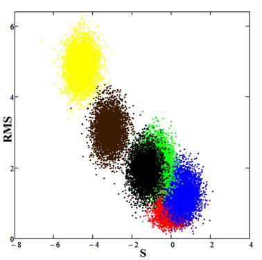
Fig.9. Red spot (calibration) corresponds to the experimental data, the blue spot is the result for parameter values E0 = 7.2, PLD = 12.7, the green spot is the result for parameter values E0 = 7.5, PLD = 12.7, the black spot is the result for parameter values E0 = 7.5, PLD = 13.0, the brown spot is the result for parameter values E0 = 7.5, PLD = 13.7, the yellow spot is the result for parameter values E0 = 8.2, PLD = 12.7.
The II-type β error and the probability that the data are not compatible with α = 0.005 were calculated (Table 5).
Analysis by the method of statistical comparison of data showed that the estimated model parameters E0 = 7.2, PLD = 12.7 provides the best description of the experimental values.
Table 5. Value of β and 1-χ
|
|
b |
1-χ |
|
E0=7.2, PLD=12.7 |
0.78 |
0.35 |
|
E0=7.5, PLD=12.7 |
0.44 |
0.71 |
|
E0=8.2, PLD=12.7 |
0 |
0.997 |
|
E0=7.5, PLD=13.0 |
0.054 |
0.969 |
|
E0=7.5, PLD=13.7 |
0 |
0.997 |
4. Conclusion
The program is based on the method for statistical comparison of data designed for visualization of the distributions obtained and for calculation of the probability that the data do not belong to the same general population. The method allows one to analyze the theoretical and experimental data, and to determine which model best describes the experimental data. Universality of the method for statistical comparison makes it possible to carry out data analysis in the tasks that require their comparison, the choice of computational models, determination of confidence intervals of the calculated model parameters within which the model is in good agreement with experiment. Visualization of the results can significantly enhance the efficiency of the analysis, giving a natural visibility of the computational procedure results.
References
1. O. Thas, Comparing Distributions, Springer Series in Statistics, 2010.
2. Bityukov S.I., Krasnikov N.V., Maksimushkina A.V., Nikitenko A.N., Smirnova V.V. Metod statisticheskogo sravnenija dannyh i ego primenenie dlja analiza jeksperimental'nyh jaderno-fizicheskih dannyh [A method for statistical comparison of data sets and its uses in analysis of nuclear physics data]. Proceedings of Universities. Nuclear Power, 2014, № 3, pp. 43-51. [In Russian]
3. Bityukov S.I., Krasnikov N.V., Nikitenko A.N., Smirnova V.V. A method for statistical comparison of histograms arXiv:1302.2651 - 2013.
4. Bityukov S., Krasnikov N., Nikitenko A., Smirnova V. Eur.Phys.J.Plus- 2013.- №128:143.
5. Bityukov S.I., Krasnikov N.V., Nikitenko A.N., Smirnova V.V. Vestnik RUDN. Seriya: matematika, informatika, fisika. 2014, no.2, p. 324. [In Russian]
6. Bityukov S.I., Krasnikov N.V., Distinguishability of Hypotheses. Nucl.Inst.&Meth. – 2004 -A534. P.152.
7. The computer program "Statistical comparison of the calculated and experimental data," the certificate of №2015614094 from 06/04/2015.
9. Korovin Yu. A., Maksimushkina A. V. Use of Neural Networks for Nuclear Data Approximation [Ispol'zovanie nejronnyh setej dlja approksimacii jaderno-fizicheskih dannyh]. Nuclear physics and engineering, vol. 5, no. 3, pp. 237-246, 2014. [In Russian]
10. https://www-nds.iaea.org/exfor/exfor.htm
11. Osovsky S. Neural networks for information processing [Nejronnye seti dlja obrabotki informacii]. Finance and Statistics, 344 pp., 2002. [In Russian]
12. Diyakonov V. Kruglov V. Matematicheskie pakety rasshirenija MatLAB. Special'nyj spravochnik [Mathematical packages of extension of MatLAB. Special handbook]. Peter, 488 pp. 2001. [In Russian]
13. http://www.mathworks.com/products/neural-network/
14. Mark Hudson Beale, Martin T. Hagan, Howard B. Demuth. Neural Network Toolbox TM User’s Guide R2013b
15. https://www-nds.iaea.org/spallations/cal/ fom_definition.pdf
16. Pashchenko A.B. et al., "FENDL/A-2.0 Neutron activation cross section data library for fusion applications", report IAEA(NDS)-173 (IAEA October 1998) https://www-nds.iaea.org/fendl/fen-activation.htm
17. Korovin Yu. A., Maksimushkina A. V., Natalenko A. A. Interaktivnaja sistema po raschetu izotopnogo sostava i navedennoj aktivnosti obluchennyh materialov perspektivnyh JaJeU [Interactive System for Calculating the Isotope Composition and Induced Radioactivity of Irradiated Materials on Nuclear Power Facilities]. Bulletin MEPhI, vol. 2, №1, p. 79-84, 2013. [In Russian]
18. Korovin Yu. A., Maksimushkina A. V. Raschet izotopnogo sostava i navedennoj aktivnosti obluchennyh materialov innovacionnyh jelektrojadernyh ustanovok [Calculation of isotopic composition and induced activity of irradiated materials in innovative accelerator-drive systems], Proceedings of Universities. Nuclear Power, no. 2, pp.51-59, 2014. [In Russian]
19. A.V. Ignatyuk, K.K. Istekov, G.N. Smirenkin, Sov. J. Nucl. Phys. 29(4) (1979) 450.