FEATURE SPACE VISUALIZATION IN THE METHOD FOR COMPACT REPRESENTATION OF CONTOURS
D.A. Borisoglebskiy1, E.V. Chepin2
1 UAB AIA, Russia
2 National Research Nuclear University MEPhI, Russia
denis.borisoglebsky@gmail.com, evchepin@gmail.com
Contents
2. Review of existing methods of shape representation for silhouettes on digital images
3. Description of the basic idea of the proposed method
4. Formulation of the problem for research of the feature space
5. Selection of the source data
Annotation
The article describes one of the approaches to solving the problem of silhouettes’ shape representation on digital images. The results of the research for developed contour-based method for representing silhouettes in the form of a sequence of parameterized primitives in terms of coverage of feature space. The results were studied by the methods of scientific visualization that made it possible to draw quick and visual conclusions about the behavior of the analyzed data and apply appropriate methods for solving the problems in the experiment. The developed method will be useful for solving practical problems of silhouettes’ shape representation in various areas of image processing.
Keywords: silhouettes’ shape representation, parameterized primitive, regression analysis, cluster analysis, visualization of multidimensional data.
1. Introduction
The method of scientific visualization (MSV) is widely used in many fields of science and technology. It is possible to identify the general problem of this scientific approach as follows: “for the initial analyzed data using a computer there is assigned some of their static or dynamic graphical interpretation that is visually analyzed and the results of the analysis of this graphic interpretation are then interpreted in relation to the original data” [25]. Fields of the MSV use can be divided into two major segments:
- Visualization of data from real physical or production units/processes.
- The visualization of data obtained as a result of model/current computational experiments.
It is important that in both cases we are talking about the fact that as a result of the MSV we get new information about the investigated process that is impossible or more difficult to obtain in other ways [25 - 26].
There are many examples of the MSV usage: visualization of nanostructures [25, 27, 31], modelling of nanoelectronics [27], 3D-modelling of radiating plasma [28], visualization in the computational fluid dynamics [29 ], geometric patterns in biology [32 - 33], visualization of geophysical problems [34], visualization of collisions of elementary particles [35, 38].
In this paper shape representation problem for silhouettes in the 2D-image is considered. This problem is not a typical task of image processing and the MSV. The purpose of this approach to image processing is to obtain compact description of the boundary contours of objects for applications that requires,, for example, the delivery of such descriptions on the data transmission with small bandwidth or storage of a large number of descriptions in the memory. It is important to note that the proposed method has inverse transformation, i.e. restores the contour of the description with acceptable accuracy. However, the computational complexity of the proposed approach is very high. The necessity arises to use parallel programming techniques and methods of processing large volumes of data (big data).
As a rule, the task of interpretation of large data sets can be easily solved if you know what kind of information you need and how to extract it. For our problem the analysis of multidimensional feature space (MFS) is reduced to cluster analysis. In this case the situation changes. On the one hand the clustering problem is solved by one of the large number of existing algorithms. On the other hand - the correctness of the results greatly depends on the information about the number of clusters. Visualization of the MFS is the quickest and easiest way to find the number of the clusters. When visualizing spaces that have more than three dimensions it is also necessary to decrease the dimension of the data. This problem occurs because the human mind cannot perceive more than three geometrical dimensions [30]. To reduce the dimensions of the data the regression analysis is used.
In many problems related to image processing the developer faces the necessity of submission of the original video in the "compressed" form. Pixel image must be submitted in the form of a structured description which contains all the important information about the features of a particular image. For example, this is usual for pattern recognition problems in the images, the tasks of computer graphics, computer vision systems, robotics, systems for "understanding" image, systems for automated production, GIS technology and many others. The classical approach to solving these problems is the theory based on the use of various types of features. It allows to transfer the solution of the problem in the space of these features [37]. This ideology is effectively working in a number of problems but it certainly does not provide complete and sufficient flexibility in tasks that allow to process complex information contained on 2D and, especially, 3D images.
This article describes a method of representing the contours in a sequence of parameterized primitives. This method is a modification of the method of semantic description of contours [1-2] which uses the ideas of K.Fu [3] on the structural description of the approach to the problem of determining the form of the empirical model [4]. The basic idea of an improved method is described in [5-10] and is reduced to the solution of two problems - contour decomposition and representation each of the fragments in the form of a parameterized primitive.
Decomposition of the contour is based on the analysis of curvature function. Selection of the primitive and its parameters determination involve the usage of normalization to each fragment of several transformations - parallel translation, scaling, rotation and mirroring of the axis. For each normalized fragment, we calculate the characteristic of a curve shape. This characteristic is called a feature vector. This approach allows to translate the search of a parameterized primitive to the MFS. The method involves preliminary training of the classifier. Training provides a set of feature vectors - points in the MFS which determine the appropriate shape of the curve feature with parameterized primitive.
The viewed method was developed in the "Robotics" laboratory of the Department "Computer Systems and Technologies" NRNU MEPhI as a part of work on a mobile robotic system (MRS) [11-14].
2. Review of existing methods of shape representation for silhouettes on digital images
The classical theory of the shape representation divides all existing approaches into two main groups. Depending on the source of information we share contour-based and region-based representations [15 – 16]. In its turn, each of the areas is divided into two groups depending on the locality of the used information structural and global approaches are distinguished. The viewed method of compact contours description is related to the structural contour approach. The contour-based approach allows us to represent the shape of the object most compactly in comparison with the region-based description. A structured approach increases the flexibility of descriptions.
There are several main groups of methods implementing the structural description of the contours: piecewise-linear approximation [17 - 18], the selection of the parameters of the primitive [19-21], the calculation of the parameters of primitives with check the accuracy of the representation [1, 22 - 23], the use of spline interpolation to the parametric representation of the contour [24], the selection of primitives and their parameters on the basis of their similarity in the MFS [2, 5-10]. Piecewise-linear approximation is a rough approximation of the contour of the impossibility of representation of smooth sections of the curve, and therefore is not suitable for all tasks. Methods with the selection of parameters for primitives are demanding in terms of computing and are limited to a small number of parameters. Spline interpolation means that the contour is represented in a parametric form – in the form of two (for a 2D contour) single-valued functions which leads to excessive description size.
Methods with the MFS are faster than methods with the selection of parameters and allow to obtain a more compact description compared to methods using spline interpolation. In view of the above-mentioned reasons there was selected a group of methods with feature space, and the considered in this article method of contours compact description is a modification of the basic method of this group - the method of semantic contours description [2].
Method of contours compact description is based on the feature space method? and the results of image contours presentation are highly dependent on how the space is used. It has been found that to obtain acceptable quality presentation the necessary dimension of a feature space need to be from 8 to 12 [10].
3. Description of the basic idea of the proposed method
The basic idea of [5-10] is reduced to contour decomposition into fragments and the presentation of each of the fragments in the form of a parameterized primitive - an analytic representation of the curve. In terms of the MFS’s research the most interesting is the second problem. Let’s consider it more as an example of three-dimensional feature space.
In the method of compact contours description of the image before calculating the elements of the feature vector contours fragment the normalization for several transformations is produced. It results in a curve with points that satisfy the condition:
![]() (1)
(1)
where ![]() - a total number of contours fragment
points,
- a total number of contours fragment
points, ![]() – a
leftmost point,
– a
leftmost point, ![]() – a
rightmost point.
– a
rightmost point.
The elements of the feature vector are calculated as the
coordinates of points on the axis ![]() ,
corresponding to values uniformly distributed along the axis of
,
corresponding to values uniformly distributed along the axis of ![]() after
normalization:
after
normalization:
![]() (2)
(2)
where ![]() - the
- the
![]() th
element of the feature vector,
th
element of the feature vector, ![]() - a dimension of the feature vector,
- a dimension of the feature vector, ![]() is
calculated as follows:
is
calculated as follows:
![]() (3)
(3)
Formation of the feature vector is produced only for
single-valued curves. The process of calculating the feature vector elements is
illustrated on Figure 1: there are chosen points on the normalized curve ![]() :
: ![]() ,
corresponding to
,
corresponding to ![]() the following coordinates on the axis
the following coordinates on the axis ![]() :
: ![]() . The
coordinates of these points that are taken along the axis
. The
coordinates of these points that are taken along the axis ![]() are
elements of the feature vector.
are
elements of the feature vector.
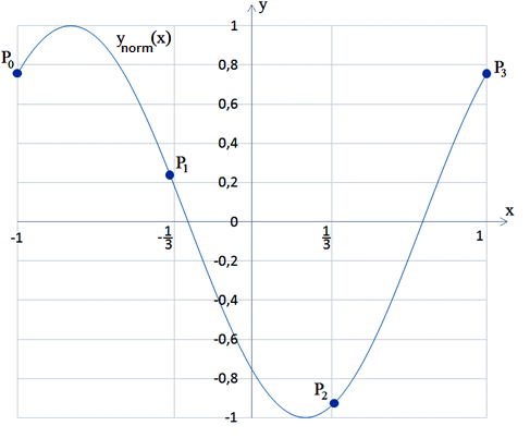
Fig.1. Formation of feature vector in the three-dimensional feature space.
Formed feature vector can be represented by a point in N-dimensional feature space that allows the visualization of sets of feature vectors for N equal or lower than 3.
4. Formulation of the problem for research of the feature space
The number of points in the MFS is defined by the vectors of features from the database of the contour fragments classifier. In its turn, the contents of the database with primitives is directly dependent on the training sample. For a given training sample the contents of the database with primitives is uniquely determined. For each feature vector from the database with primitives in the MFS the appropriate shape of the curve (feature vector - shape descriptor) and the analytic representation of the curve are defined. This correspondence is defined in the locality of the feature vector for a given accuracy. A set of N-dimensional volume of space (area for 2 dimensions, volume - for 3, etc.) which are defined in accordance with the specified accuracy will be called coverage of the MFS. The ratio of space coverage features to all N-dimensional volume of space is the degree of coverage. If the MFS is completely covered, that is there is no point that does not determine the appropriate feature vector with the analytic representation of the curve, such coverage will be called complete.
Under the miss we mean a situation where a match in the MFS within a given accuracy for some feature vector is not found. Thus the presence of misses in the contour impairs compact description by increasing the number of contours fragments. So there occurs need to increase the coverage of the MFS.
Ideally, the feature space should have full coverage, on the other hand, the coating will be provided either by large errors or due to a large number of points which is not applicable in practice. Therefore instead of full coverage it is expedient to cover the most popular points
Under the popular points
to a set of input data (contours) we mean the set of feature vectors for which
in the process of the contour description there is searched the accordance to
the analytic representation of the curve. In this paper the value that characterizes
a certain amount ![]() of popular points coverage is
interesting:
of popular points coverage is
interesting:
![]() , (4)
, (4)
where ![]() – a current number of popular points;
– a current number of popular points;
![]() – a
total number of all popular points.
– a
total number of all popular points.
Thus, the set of primitives in a database in MFS should cover certain specified proportion of popular feature vectors within a given accuracy. Since the set of primitives depends directly on the training sample the problem takes the following form.
For some of the input data set it is necessary to choose such a training sample which will provide coverage of the given proportion of popular feature vectors in the MFS. To accomplish this you must solve several subtasks: select inputs, develop a scheme of the experiment and make an experiment.
5. Selection of the source data
As the data for the experiment there was used a base of binary images obtained from clipart images which are freely available on the Internet.
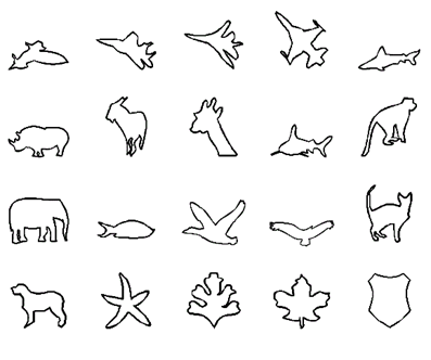
Fig. 2. An example of contours obtained from the database of images.
The clipart implied image is the image from the set of silhouettes with one theme as a rule (Figure 2). In total, the images created from the database consist of 745 binary images from which you can extract exactly one contour as the original binary image containing the connected area without openings. It should be noted that the presence of only one contour of the image is selected for the convenience of the experiment and is not a limitation of the method.
6. Scheme of the experiment
For this experiment there was selected a dimension of
feature vector corresponding to the dimensions of the MFS recommended for work
with real images [10] - ![]() . As an error of data there was taken a
deviation of reference points from the reconstructed corresponding points of
the initial contour of no more than 5 pixels. The critical value of proportion
coverage for popular feature vectors of the total number of points in the MFS,
to which the experiment was carried out, was taken as follows:
. As an error of data there was taken a
deviation of reference points from the reconstructed corresponding points of
the initial contour of no more than 5 pixels. The critical value of proportion
coverage for popular feature vectors of the total number of points in the MFS,
to which the experiment was carried out, was taken as follows:
![]() (5)
(5)
Thus, the experiment is terminated if the condition:
![]() (6)
(6)
is fulfilled.
First, there is the need to determine the total number of popular points in the MFS. For this first stage of the experiment the processing of all contours of base image without learning classifier of contours fragments was carried out. Since the training set was empty, the database with primitives does not contain any records. Thus, all the misses in the MFS in this case are popular feature vectors of the image database.
The second and subsequent stages of the experiment imply the following steps:
· Teaching the classifier of contours fragments using the training sample.
· Determining a set of misses in the MFS for the training sample.
· The conclusion about the need to improve the coverage for popular points in the MFS. If the improvement for popular points coverage is necessary then:
o Determination of the number of alleged clusters.
o Clustering sets of misses with validation of decomposition using visualization.
o Getting of reference points for all primitives feature vectors corresponding to the centers of clusters.
o Selection of a parameterized primitive for each set of reference points.
o Updating the training sample.
Thus, the result of the experiment is a training sample, providing coverage for more than 95% popular points as required for the task.
7. Experiment
Step 1. Getting the total number of popular points. Contour processing was made from the base image without training the classifier for contours fragments. As a result the misses were registered:
![]() (7)
(7)
It should be noted that the results misses correspond to the required popular points:
![]() (8)
(8)
In every step of the experiment this value allows to determine the ratio of the popular points in the feature space of the total number by the formula (4).
Step 2. Investigation of points in multidimensional feature space without learning classifier for contours fragments.
In Step 1 there has been received a set of the popular points which at this stage corresponds to misses in feature space to be tested:
![]() (9)
(9)
According to the scheme of the experiment the research of this set involves visualization. It results in need to reduce the dimensionality of data, for this purpose one of regression analysis methods - the principal component analysis (PCA) [36] is the most suitable.
PCA reveals the relationship between the variables and presents the data in the new basis of lower-dimensional representation with the possibility to control error. The output data of the method is the matrix scores and loadings. Matrix scores - is a projection of the original data to the subspace of the principal components. Matrix of loadings allows to go from the original space of variables to the space of the principal components and vice versa. Decomposition of the initial data into the components of the method of principal component analysis is consistent and iterative process that can be terminated at any step. To assess the accuracy of the representation of the original set of points with the help of a number of components there is used a matrix of remnants - the difference between the original matrix and the one resulting from the description by a component. Evaluation of dispersion ith point in N-dimensional space:
![]() (10)
(10)
where ![]() - the
element of the matrix remnants.
- the
element of the matrix remnants.
The total estimate of the variance of all the K popular points becomes:
![]() (11)
(11)
The standard means of Statistica can automatically plot the accuracy of the representation of the set the popular points by a number of components (Figure 3). From this graph it is clear that most of the information is contained in the first 3-4 components.
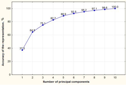
Fig. 3. Graph of the representation accuracy of the set of the popular points on the number of components.
For visualization of the original set of points in space component it is more convenient to use three components which corresponds to 75.1% of the data modeling. To evaluate the visual presence of clusters in three-dimensional space it is necessary to consider 3-dimensional "cloud" of points with different angles. Therefore, there is the need for rotation of visualized data. For these purposes the Statistica software package was used, whereby there was obtained a three-dimensional space first component visualization (Figure 4). The visualization provides the only marked accumulation of points, therefore, the cluster analysis of the set of points for the further analysis, in this case, it is not required. The same conclusions can be drawn after the visualization of 2 components (with accuracy 64.5%) – figure 5.
Fig. 4. Visualization of three-dimensional space component at the 2nd step of the experiment.
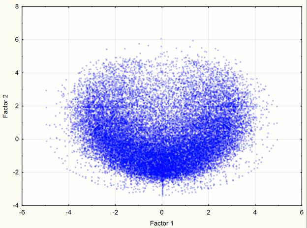
Fig. 5. Visualization of two-dimensional space component at the 2nd step of the experiment.
The presence of only one cluster eliminates the calculation of the center as the average of the coordinates of all the popular points of the initial set. The results are shown in Table 1.
Table 1. The coordinates of the cluster center of the original set
|
i |
0 |
1 |
2 |
3 |
4 |
5 |
6 |
7 |
8 |
9 |
|
v |
0,70 |
0,26 |
-0,02 |
-0,21 |
-0,33 |
-0,36 |
-0,32 |
-0,21 |
-0,02 |
0,26 |
Axis coordinates ![]() in
Table 2 were obtained by (3) from the geometric meaning of the feature vector -
a point in the MFS.
in
Table 2 were obtained by (3) from the geometric meaning of the feature vector -
a point in the MFS.
Table 2. A geometric interpretation of the feature vector corresponding to the center of the cluster from Table 1.
|
x |
-1 |
-0,8 |
-0,6 |
-0,4 |
-0,2 |
0 |
0,2 |
0,4 |
0,6 |
0,8 |
1 |
|
y |
0,70 |
0,26 |
-0,02 |
-0,21 |
-0,33 |
-0,36 |
-0,32 |
-0,21 |
-0,02 |
0,26 |
0,70 |
According to Table 2 there was constructed a primitive fragment contour corresponding to the feature vector from the cluster center of points in the MFS (Figure 6).
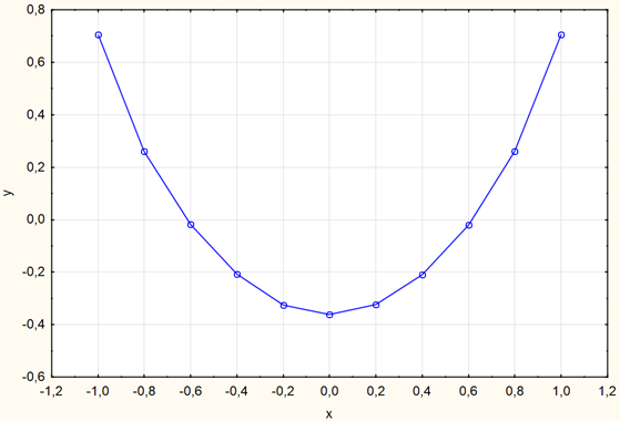
Fig. 6. Primitive of fragment of contour at the 2nd step of the experiment according to Table 2.
The form of the primitive in Figure 5 shows that the most popular primitive is the arc so this primitive will be added to the training set.
Step 3 Investigation of popular points in the MFS with the training of the classifier for contour fragments of one class of primitives.
At this stage, there have also been processed contours from the image database but this time the classifier of contour fragments has been trained on the family of arcs. Since much of the popular points became covered with feature vectors corresponding to the family of arcs the number of misses was reduced:
![]() (12)
(12)
According to the formula (4) the ratio of popular covered points approximately equals to:
![]() (13)
(13)
For this value the termination condition (7) is not satisfied so the research of the MFS was continued. By analogy with the preceding step to visualize the received data there has been applied a method of regression analysis - PCA. Visualization of three-dimensional and two-dimensional component space at this stage is shown in Figures 7-8.
Fig. 7. Visualization of three-dimensional component space at the 3rd step of the experiment.
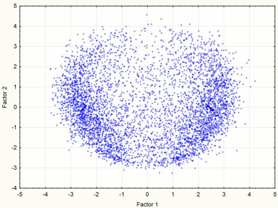
Fig. 8. Visualization of two-dimensional component space at the 3rd step of the experiment.
Visualization has identified two obviously expressed sets of points so it became necessary to use methods of cluster analysis. For this work we used the method of clustering K-means which gives good results if you know the required number of clusters. To check the correctness of the decomposition of the original set of points in the group there was held the visualization after data clustering (Figures 9 - 10). These images confirm the correctness of the decomposition.
Fig. 9. Visualization of three-dimensional space component at the 3rd step after clustering.
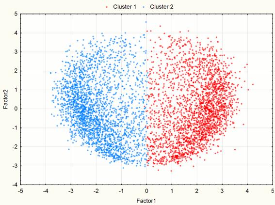
Fig. 10. Visualization of two-dimensional space component at the 3rd step after clustering.
Thereafter there were determined center coordinates of each cluster to obtain a characteristic shape for popular primitives. Coordinates of centers have been calculated as an average of points’ coordinates for each cluster, the results of the calculations are shown in Table 3.
Table 3. Coordinates of the cluster centers for the set of points corresponding to the misses at the 3rd stage of the experiment.
|
i |
0 |
1 |
2 |
3 |
4 |
5 |
6 |
7 |
8 |
9 |
|
Cluster 1 |
0,62 |
0,64 |
0,56 |
0,40 |
0,13 |
-0,15 |
-0,41 |
-0,55 |
-0,50 |
-0,16 |
|
Cluster 2 |
0,62 |
-0,13 |
-0,49 |
-0,54 |
-0,40 |
-0,15 |
0,16 |
0,41 |
0,56 |
0,62 |
According to the geometrical interpretation of points in the MFS and formula (3) there were obtained the approximate points through which the most popular primitives pass at this stage of the experiment for each cluster (Table 4).
Table 4. Geometrical interpretation of feature vectors corresponding to the centers of clusters in Table 3.
|
i |
0 |
1 |
2 |
3 |
4 |
5 |
6 |
7 |
8 |
9 |
0 |
|
x |
-1 |
-0,8 |
-0,6 |
-0,4 |
-0,2 |
0 |
0,2 |
0,4 |
0,6 |
0,8 |
1 |
|
y1 |
0,62 |
0,64 |
0,56 |
0,40 |
0,13 |
-0,15 |
-0,41 |
-0,55 |
-0,50 |
-0,16 |
0,62 |
|
y2 |
0,62 |
-0,13 |
-0,49 |
-0,54 |
-0,40 |
-0,15 |
0,16 |
0,41 |
0,56 |
0,62 |
0,62 |
Constructed contour fragment primitives are shown in Figure
11. Visualization of the results allowed us to see the symmetry of primitives
relative to the axis ![]() .
Considering that this contour representation method in encoding of contour
fragments provides invariance including mirroring transformations there was
obtained a conclusion about the necessity of only one primitive. The shape of
the normalized curve with the forming method allowed to come to a conclusion
about the original analytic representation of the primitive - sine wave taken
in the interval
.
Considering that this contour representation method in encoding of contour
fragments provides invariance including mirroring transformations there was
obtained a conclusion about the necessity of only one primitive. The shape of
the normalized curve with the forming method allowed to come to a conclusion
about the original analytic representation of the primitive - sine wave taken
in the interval![]() . For
the training it was decided to use sample family of sine waves which increased
the coverage of popular feature vectors.
. For
the training it was decided to use sample family of sine waves which increased
the coverage of popular feature vectors.
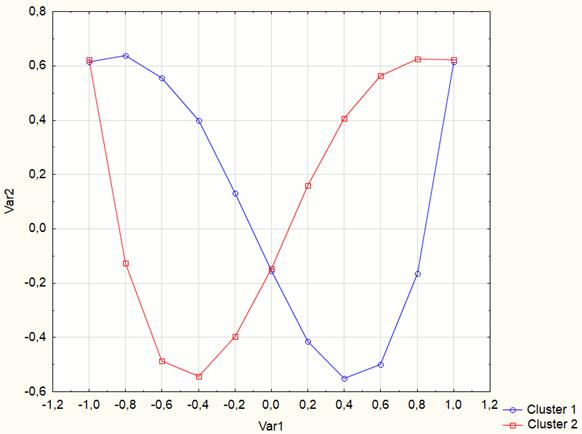
Fig. 11. Primitives for contours fragments at the 3rd stage of the experiment according to Table 4.
Step 4. Investigation of the MFS with the training of the classifier of contour fragments for two classes of primitives.
This time in the training sample there are 2 classes of curves - arcs and sine waves. Contours processing from the image database showed that the number of misses after the last change of training sample was reduced:
![]() (14)
(14)
According to the formula (4) the ratio of covered popular points approximately equals to:
![]() (15)
(15)
Thus, the condition of the experiment completion (6) is satisfied, so the current training set consisting of two classes of curves is the required one.
8. Conclusions
Using scientific visualization in the problem allows to examine the behavior of the test data quickly and clearly and to apply the developed approach to solving the problem of object contour description in the images in practice. In this paper there was demonstrated the application of scientific visualization methods for research of the MFS used in the recognition of non-linear functions from the basis for describing the object contours in the image. As it is shown previously, to obtain rough estimates of the cluster number we can quickly get the information which is difficult to obtain with analytical methods in practical use.
It should be noted that the presented approach using MSV is
suitable for different boundary conditions. Conditions ![]() , N=10
were selected taking into account the characteristics of the method and not
because of the MSV limitations. Also, the presence of only two clusters
(Figures 9-10) is a particular case, the proposed approach would do well to any
small number of clusters in MFS and this number cannot be large because of the
conditions of the task.
, N=10
were selected taking into account the characteristics of the method and not
because of the MSV limitations. Also, the presence of only two clusters
(Figures 9-10) is a particular case, the proposed approach would do well to any
small number of clusters in MFS and this number cannot be large because of the
conditions of the task.
The results suggest that the methods of visual analysis of the big data are quite effective in practical use for such non-traditional problem for the given scientific method.
9. Software
The system of encoding/decoding contours has been implemented in C ++ using OpenCV library. Statistical analysis of the results was considered for the following software: Matlab, OriginPro, Statistica. A study of data in multi-dimensional feature space data involves the use of cluster analysis and regression analysis, and visualization of data being processed. All these features are present in each of these products. Statistica software was used in the research described in this article.
Bibliography
- D.K. Fedorov, E.V. Chepin. Algoritmy raspoznavanija obrazov na osnove atributnyh grammatik dlja cifrovoj obrabotki izobrazhenij [Pattern recognition algorithm based on attribute grammars for digital image processing]. Moscow, Preprint of MEPhI, 1988; [In Russian]
- Lepeshenkov K.E., Tchepine E.V. Semantic Editor of 2-d Contour Images. Proceedings of Intern. Conf. “GraphiCon’99”, Moscow, 1999;
- Fu K. Strukturnye metody v raspoznavanii obrazov [Syntactic Methods in Pattern Recognition]. Academic Press, 1974; [In Russian]
- Katashkin V.I., Levahin M.G., Chepin E.V. Ob odnom podhode k resheniju zadachi opredelenija vida jempiricheskoj modeli [An approach to solving the problem of determining the type of empirical model]. Engineering and mathematical methods in cybernetics, 1979, №8; [In Russian]
- Borisoglebskiy D.A. Improve parametric curves representations in the semantic description of contours. Proceedings of the 14th International Workshop on Computer Science and Information Technologies, vol. 1, Hamburg, 2012;
- Borisoglebskiy D.A., Chepin E.V. Opisanie usovershenstvovannogo metoda predstavlenija kontura v vide posledovatel'nosti parametricheskih krivyh [Description of an improved method of contour representation in the form of a sequence of parametric curves]. Proceedings of the VII International scientific-technical conference "Automation and advanced technologies in the nuclear industry", Novouralsk, 2012; [In Russian]
- Borisoglebskiy D.A. Rassmotrenie odnogo iz jetapov usovershenstvovannogo metoda semanticheskogo opisanija konturov na primere mobil'nogo robototehnicheskogo kompleksa [Consideration of one of the stages of an improved method of semantic contour description on the example of a mobile robotic system]. Proceedings of the 55th scientific conference of MIPT, Moscow, 2012; [In Russian]
- Borisoglebskiy D.A. Sistema formirovanija kompaktnogo opisanija konturov izobrazhenija [The system of formation of a compact description of image contours]. Proceedings of the 16th international telecommunication conference of young scientists and students "Youth and Science", Moscow, 2013; [In Russian]
- Borisoglebskiy D.A., Chepin E.V. Usovershenstvovannyj podhod k zadache vektorizacii konturov na izobrazhenijah [An improved approach to the problem of vectorization of contours in images]. Applied Informatics no. 44 (2), Moscow, 2013; [In Russian]
- Borisoglebskiy D.A. Vlijanie modifikacii metoda semanticheskogo opisanija konturov na harakteristiki podsistemy robototehnicheskogo kompleksa [Effect of modification in the method of semantic contour description on the characteristics of the subsystem robotic system]. Applied Informatics, no. 48 (6), Moscow, 2013; [In Russian]
- Chepin E.V., Dyumin A.A., Shapovalov N.K., Sorokoumov P.S. Hardware and Software of Mobile Robots Group. Proceedings of the International Workshop on Computer Science and Information Technologies. Hamburg, 2012;
- Danilov V.V., Dyumin A.A., Sorokoumov P.S., Chepin E.V., Shapovalov N.K. Programmnaja sistema distancionnogo upravlenija robotom PATROLBOT [Software system of remote control of PATROLBOT robot]. Proceedings of the "Science and Innovation MEPhI", Moscow, 2010; [In Russian]
- Dyumin A.A. Architecture of reconfigurable software for mobile robotic systems. Proceedings of the 12th International Workshop on Computer Science and Information Technologies, vol. 2, Crete, 2009;
- Dyumin A.A., Sorokoumov P.S. Arhitektura sistemy upravlenija komandoj mobil'nyh robotov [The architecture of system to control a team of mobile robots]. Proceedings of the 54th scientific conference of MIPT, Moscow, 2011; [In Russian]
- Dengsheng Zhang, Guojun Lu. Review of shape representation and description techniques. Pattern Recognition, №37, 2004;
- Luciano Da Fontoura Costa, Roberto Marcondes Cesar Jr. Shape Analysis and Classification: Theory and Practice, 2000;
- Kolesnikov A., Franti, P. Polygonal approximation of closed discrete curves. Pattern Recognition, no. 40, 2007, pp. 1282-1293;
- Alexander Kolesnikov, Fränti Pasi, Bigün Josef (Bearb.), Gustavsson Tomas (Bearb.). Polygonal Approximation of Closed Contours. 2749. In: SCIA: Springer, 2003 (Lecture Notes in Computer Science). ISBN 3-540-40601-8, pp. 778-785;
- Shirma A.A. Nejrosetevaja approksimacija vektornyh ob#ektov krivymi Bez'e [Neural network approximation of vector objects using Bezier curves]. Neuroinformatics, 2011; [In Russian]
- Belyh S.V. Approksimacija geometrii kontura dugami pri kontrole tochnosti izgotovlenija detalej letatel'nyh apparatov [Approximation of the geometry of the circuit using arcs in the control of precision manufacturing of aircraft details]; [In Russian]
- Levashov, Yurin. Sistema bystrogo obnaruzhenija parametricheskih krivyh [System of quick detection of parametric curves]. Graphicon, 2011; [In Russian]
- Vishnevskiy V.V., Kalmykov V.G. Strukturnyj analiz cifrovyh konturov izobrazhenij kak posledovatel'nostej otrezkov prjamyh i dug krivyh [Structural analysis of digital contours in the images as a sequence of line segments and arcs of curves]. Artificial Intelligence, №3, 2004; [In Russian]
- Kalmykov V.G. Strukturnyj metod raspoznavanija otrezkov cifrovyh prjamyh i konturnyh binarnyh izobrazhenij [Structural method for recognizing segments of digital lines and binary contour images]. Artificial Intelligence, №2, 2002; [In Russian]
- Myazina U.S., Lisienkova L.N. SAPR Odezhdy [CAD for clothing], 2007;
- Strikhanov M.N., Degtyarenko N.N., Pilyugin V.V., Malikova E.E., Matveeva M.N., Adzhiev V.D., Pasko A.A. Opyt komp'juternoj vizualizacii nanostruktur v NIJaU MIFI [Computer visualization of nanostructures experience at NRNU "MEPhI"]. Scientific Visualization, vol. 1, no. 1, 2009, pp. 1–18; [In Russian]
- Pasko A.A., Pilyugin V.V. Nauchnaja vizualizacija i ee primenenie v issledovanijah nanostruktur [Scientific visualization and its application in the research of nanostructures]. Rusnanotech, Nanotechnology International Forum, Abstracts of reports of scientific and technical sections. 2008, Moscow, pp. 189-190; [In Russian]
- Polyakov S.V., Iakobovski M.V. Geometricheskoe modelirovanie i vizualizacija v zadachah sovremennoj jelektroniki [Geometrical simulation & vizualization in problems of modern electronics]. Scientific Visualization, vol. 1, no. 1, 2009, pp. 19-65; [In Russian]
- Kartasheva E.L., Bagdasarov G.F., Boldarev A.S., Gasilova I.V., D S.V.'yachenko, Olkhovskaya O.G., Shmirov V.A., Boldyrev S.N., Gasilov V.A. Vizualizacija dannyh vychislitel'nyh jeksperimentov v oblasti 3D modelirovanija izluchajushhej plazmy, vypolnjaemyh na mnogoprocessornyh vychislitel'nyh sistemah s pomoshh'ju paketa Marple [Scientific visualization of data from parallel supercomputer 3D radiative plasma simulations implemented using code Marple]. Scientific Visualization, vol. 2, no. 1, 2010, pp. 1-25; [In Russian]
- Bondarev A.E., Galaktionov V.A., Chechetkin V.M. Nauchnaja vizualizacija v zadachah vychislitel'noj mehaniki zhidkosti i gaza [Scientific visualization for computational fluid dynamics]. Scientific Visualization, vol. 2, no. 4, 2010 pp. 1 – 26; [In Russian]
- Vasev P.A., Perevalov D.S. O sozdanii metodov mnogomernoj vizualizacii [About creation of methods for multidimensional visualization]. Graphicon 2002, pp. 431–437; [In Russian]
- Bagaturyants A.A., Vladimirova K.G., Degtyarenko N.N., Malikova E.E., Minibaev R.F., Pilyugin V.V., Strikhanov M.N., Freidzon A.Y. Vizualizacija i konstruirovanie nanosistem v ramkah mnogomasshtabnogo podhoda: programma «Nanomodeller» [Visualization and design of nanostructures in multiscale approach: “Nanomodeller” program]. Scientific Visualization, vol. 2, no. 4, 2010, pp. 40-60; [In Russian]
- Bojenko V.K., Ivanov A.O., Mishchenko A.S., Tuzhikin A.A., Schyschkin A.M. Geometricheskie modeli v biologii: kak i chto mozhno modelirovat' [Geometrical models in biology: what and how we can simulate]. Scientific Visualization, vol. 1, no. 1, 2009, pp. 66-99; [In Russian]
- Konstantinov I.N., Stefanov Y.E., Kovalevsky A.A., Voronin Y.N. Trehmernaja model' VICh: graficheskij obzor dannyh o stroenii virusnoj chasticy [Three-dimensional Model of HIV: a Graphical Review of the Viral Particle Structure]. Scientific Visualization, vol. 3, no. 1, 2011, pp. 53-54; [In Russian]
- Larichev V.A., Lesonen D.N., Maksimov G.A., Podyachev E.V., Derov A.V. O podhode k trehmernomu matematicheskomu modelirovaniju slozhnoj geologicheskoj sredy s razryvami dlja vizualizacii i reshenija prjamyh i obratnyh zadach geofiziki [About approach to 3D mathematical modeling of complex geological medium with a discontinuity for visualization and decision of direct and inverse problems of geophysics]. Scientific Visualization, Vol. 2, №2, 2010, pp. 20-33; [In Russian]
- Borodina E.I. Kontrol', monitoring i vizualizacija dannyh jeksperimenta COSY-TOF v rezhime real'nogo vremeni [Control, monitoring and visualization of COSY-TOF experiment in real time], Abstract of the candidate of technical sciences, Moscow, 2011, 20 p; [In Russian]
- Principal component analysis: http://rcs.chemometrics.ru/Tutorials/pca.htm
- Introduction to statistical learning http://www.recognition.mccme.ru/pub/RecognitionLab.html/sltb.pdf
- Gertsenberger K., Merz S., Chepin E. Vizualizacija sobytij jeksperimenta MPD kollajdera NICA dlja sistemy monitoringa [Event Visualization of the MPD Experiment at the Nica Collider for the Monitoring System]. Scientific Visualization, vol. 6, no. 1, 2014, pp. 1–19; [In Russian]