SURVEY OF APPROACHES TO MULTIDIMENSIONAL DATA GEOMETRIZATION IN THE ANALYSIS USING COMPUTER VISUALIZATION
V.V. Pilyugin1, A.A. Pasko2, I.E. Milman1
1National Research Nuclear University MEPhI (Moscow Engineering Physics Institute), Moscow, Russian Federation
2National Centre for Computer Animation, Bournemouth University, Bournemouth, United Kingdom
VVPilyugin@mephi.ru, apasko@bournemouth.ac.uk, igalush@gmail.com
Content
2. Multidimensional spaces of analytic geometry
Abstract
During the analysis of various data using computer visualization, the visualization pipeline often contains the geometrization stage of this data using some multidimensional geometric space. In this article, we consider issues of a rational choice of a class of multidimensional spaces for the analysis of input data by the method of computer visualization.
Keywords: geometrization, geometric space, multidimensional space, computer visualization, multidimensional data, affine space, linear space
1. Introduction
As shown in work [1], during the analysis of scientific data using computer visualization, the visualization pipeline often contains the geometrization (geometric modeling) stage of this data using some multidimensional geometric space. It is important to note that this is not only true for the case of analysis of scientific data, but while analyzing data of any nature using the method of computer visualization.
Such a multidimensional geometric space basically may be any of those known in mathematics numerous geometric spaces. Each of these spaces represents a set of certain objects, which are called points [2]. These spaces are distinguished from each other by the nature of the objects contained in them as well as by their specific geometric properties. In this survey, we consider issues of a rational choice of such a space for the analysis of input data by the method of computer visualization.
2. Multidimensional spaces of analytic geometry
The choice of the multidimensional geometric space is done by the user in the context of their objectives for the analysis of initial data. However, in general, the selected geometric space has to satisfy the following basic requirements:
- simplicity and ease of transition from initial data to the taken into consideration geometric objects;
- openness of the geometric space in terms of the possibility of varying complexity and possessed geometric properties;
- simplicity of implementation (modeling) on the computer of the geometrization as a step of the initial data visualization algorithm.
Multidimensional spaces of analytic geometry are generally saisfying these requirements. The geometric space of multidimensional analytic geometry is defined as a set of points associated with one of linear spaces [3].
Linear spaces are introduced into consideration in linear algebra and are defined as sets of elements of one nature or another with the relation of equality and operations of addition and multiplication by a number corresponding to the appropriate axioms. Elements of linear spaces are called vectors. Space of real numbers, space of geometric vectors, matrices space or space of continuous functions can serve as examples of linear spaces. Affine spaces are the simplest multidimensional spaces of analytic geometry. Spaces of multidimensional analytic geometry corresponding to linear ones and, in particular, affine spaces are defined by some rules that specify the mapping of each pair of points to the corresponding vector and satisfy so-called point-to-vector axiomatics [3].
Let U be an affine space, linked to linear space L.
Points of affine space we will denote by capital letters of the Latin alphabet,
vectors of the linear space - by small letters of that alphabet. For a pair of
points A, B linked to vector x, we will write ![]() . In this
case
. In this
case ![]() is just new designation of x, as it
common in analytic geometry. The first of two points is called the start of
vector
is just new designation of x, as it
common in analytic geometry. The first of two points is called the start of
vector ![]() , second called its the end.
, second called its the end.
Mentioned above point-to-vector axiomatics includes two axioms:
1. for each point А from U and each vector x from L exists one and only one dot B from U such that ;
2.
if ![]() ,
, ![]() ,
, ![]() , where
, where ![]() – is sum of
vectors x and y.
– is sum of
vectors x and y.
The affine space U called real or complex, finite or infinite depending on whether real or complex, finite or infinite is the corresponding linear space L. An important characteristic of affine space U is its dimension, which is the number equal to the dimension of the linear space L. Respectively under the multi-dimensional affine space U we mean an affine space of dimension greater than three.
An example of affine space that is associated with a linear space, can serve as a three-dimensional affine space, which is mapped in such a way as it is done in the elementary analytic geometry with the set of geometric vectors, which, as we noted earlier, is a linear space.
In general, the affine space U and the corresponding
linear space L represent two different sets. However, we note that any
linear space L can be at the same time viewed as an affine space U [3].
It is enough to call vectors points and each pair of vectors a, b,
considered as points of U, assign a vector ![]() belonging to L. If we
denote the fact that the consideration of the vector x as a point of X
as
belonging to L. If we
denote the fact that the consideration of the vector x as a point of X
as ![]() , then this way of defining affine space can be
presented as follows:
, then this way of defining affine space can be
presented as follows:
 (1)
(1)
An important conclusion is that with this method of setting affine space, simplicity and ease of use for the purposes of geometric modeling is defined by simplicity and ease of use of the original linear space.
An important property for us of affine spaces well-known
method and simplicity in the definition of the coordinate system in these
spaces. The coordinate system in an affine space U of dimension n
is defined as follows. In this space, an arbitrary point O, called the
origin, is chosen and a basis of vectors e1,…,en
is fixed in the corresponding linear space L. Let M be an
arbitrary point in U. However, it together with the origin define the
vector ![]() belonging to L, which is called the
radius vector of the point M. Expanding the radius vector in the basis e1,…,en,
we get:
belonging to L, which is called the
radius vector of the point M. Expanding the radius vector in the basis e1,…,en,
we get:
![]() (2)
(2)
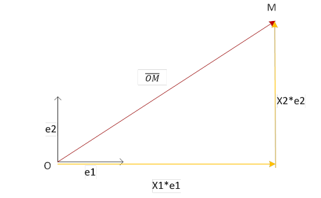
Fig. 1. Setting the affine coordinates in the basis of geometric vectors e1, e2
The coefficients of this expansion x1,…,xn
are called affine coordinates of the point M (relative to the
selected system with the origin O and the basis e1,…,en).
Let us note that the affine coordinate system is defined, in general, by two
dissimilar objects - the point O of the affine space and a basis e1,…,en
of the linear space. Obviously, in case where the linear space at the same time
viewed as affine, these objects become homogeneous, i.e., the coordinate system
determined by (n + 1) vectors of the linear space. From the theory of
linear spaces is known that the decomposition of each vector on a fixed basis
is unique, i.e., there is a single set of coordinates. Therefore, the affine
coordinates of each point are uniquely determined by the uniqueness of the
decomposition of the vector ![]() in the basis e1,…,en.
in the basis e1,…,en.
The mapping ![]() assigning to each pair of points A, B of
affine space U vector x of the linear space L, allows us
to simply and naturally analyze in affine spaces relative position of points
and on this basis make selection of geometric objects, i.e., some subsets of
points of this space, as well as to analyze the mutual arrangement of geometric
shapes.
assigning to each pair of points A, B of
affine space U vector x of the linear space L, allows us
to simply and naturally analyze in affine spaces relative position of points
and on this basis make selection of geometric objects, i.e., some subsets of
points of this space, as well as to analyze the mutual arrangement of geometric
shapes.
For example, a plane of one or another dimension which is the basic object in the affine space is defined as follows. Suppose that an arbitrary point A is fixed in the n-dimensional affine space U and arbitrary r dimensional subspace L' is fixed.
The set of all points of the affine space M for which
![]() belongs
to L' is called r-dimensional plane passing through the point A
in the direction of the subspaces L'. It is also said that L' is
a guiding subspace for the plane. The point M is called the current
point on the plane. In the definition of the plane, point A is
highlighted, but we can show that all points of the plane are equal, i.e., any
other point belonging to a given plane may play the role of point A.
belongs
to L' is called r-dimensional plane passing through the point A
in the direction of the subspaces L'. It is also said that L' is
a guiding subspace for the plane. The point M is called the current
point on the plane. In the definition of the plane, point A is
highlighted, but we can show that all points of the plane are equal, i.e., any
other point belonging to a given plane may play the role of point A.
Important special cases of the plane are a point (zero-dimensional plane), a straight line (one-dimensional plane), a hyperplane ((n-1)-dimensional plane), the entire space (n-dimensional plane). In this relation concepts such as intersecting, parallel and skew plane are introduced in affine spaces. On the basis of the plane, it is quite simple to introduce more complex geometric shapes - half-space, polyhedra, parallelepipeds and others [3].
Another important property of affine spaces, from the point of view of their use for the purposes of geometric modeling is the ability to put in one linear geometric objects as well as operations performed on them, analytical description, or, as it is said, analytically describe these objects and transformations.
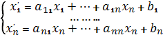
In the theory of multi-dimensional affine spaces, it is proven that the previously mentioned planes of such spaces can be placed in the appropriate analytical description using affine coordinates of points belonging to these planes. In particular, it is known that in n-dimensional affine space U and in any affine coordinates each plane S with dimension of m can be defined by a system of linear equations [3]:
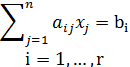 (3)
(3)
and rank r = n-m, where xj - coordinates of a point belonging to the plane. This system of linear equations is an analytical description of the plane S in the sense that the coordinates of any point belonging to this plane, are the solution of this system, but on the contrary, the coordinates of any point that does not belong to this plane, are not the solution of this system. In the transition to a new affine coordinates the type of considered linear equations change. In addition, the plane S at a fixed affine coordinate system can be described by different systems of equations. Geometrically, this means that the plane S can be defined as the intersection of various sets of the independent hyperplanes among n-m. Hyperplanes independence should be understood in the sense that the rank of a joint system of equations of these hyperplanes is the maximum possible value, i.e., is the number of equations (r = n-m).
In multidimensional analytic geometry, There are also defined analytical descriptions of other, more complex geometric shapes - polyhedra, parallelepipeds, and so on. These are the descriptions of those or other derivatives resulted from above analytical description of the planes.
It should also be noted that the analytical description of
geometric objects does not have to be based on coordinates, i.e., built using
the coordinates of the points xi, i = 1, ..., n,
belonging to these objects. These analytical descriptions can also be the
vector based, i.e., constructed using elements of the linear space that is
associated with the affine space. For example, for the hyperplane, a coordinate
analytical description for which is a linear equation of the form 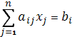 ,
the vector analytic description will be vector equation of the form:
,
the vector analytic description will be vector equation of the form:
a(x)=c (4)
where:
a(x) - a linear form, i.e., a linear numerical function of a vector argument,
x - the radius vector of a point belonging to the hyperplane
c - a constant.
From the theory of multidimensional analytic geometry it is known that other geometric objects of affine spaces can be associated with their vector analytical descriptions and the operations on geometric objects in affine spaces can be also described analytically.
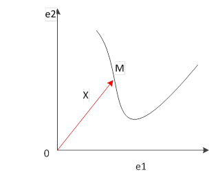
Fig. 2. Defining an object by using the radius vector in the space of geometric vectors with basis e1, e2
For example, the operations specified in the form of so-called affine transformations, the hallmark of which is the fact that the affine transformation any plane of dimension k goes to the plane of the same dimension can be associated as an analytical description of the following relationships [3]:
 (5)
(5)
It is assumed that the n×n-matrix is non-singular, ie. Det A ≠ 0. These are analytic descriptions of the operation of the affine transformation in the sense that they bind values of affine coordinate xi and xi', i=1, 2, ..., n, of corresponding to each other input and output points of geometric objects.
The concepts used in multidimensional analytic geometry (as, follows from the above material) and, in particular, the analytical description of geometric shapes and operations performed on them in many ways resemble familiar to us and evident concepts from the course of elementary analytic geometry. However, the concepts of multidimensional analytic geometry are more complex and diverse and have more abstract character.
If introduced into consideration by the user, the source data geometrization procedure involves operations of location and using different metric concepts, such as the distance between points, the length of lines, angles, and so on, then the multidimensional affine space viewed by us so far, can not be used for the purposes of geometric modeling. The fact is that unlike the space being studied in elementary geometry there are not predefined metric concepts in these spaces.
In that case, it is necessary to use other, more complex multidimensional space of analytic geometry. However, it is important to emphasize that these spaces are not opposed to affine one and can be obtained by completions with well-known and relatively simple way of introducing the necessary metric concepts. This demonstrates one of the most important in terms of geometric modeling properties of multidimensional spaces of analytic geometry. From the viewpoint of modeling these spaces can be considered as some common geometric environment with variable functionality.
The basic metric concept is the distance between points. This concept, as well as other concepts of multidimensional spaces of analytic geometry is defined by a linear space L, the associated affine space U. A new operation of scalar multiplication of vectors is introduced into the space L to do that. Scalar multiplication assigns to each pair of vectors x, y in L a real number, which is denoted by (x, y) and called the scalar product of x by the vector y. The rule by which a real number is assigned to arbitrary pair of vectors may be arbitrary, but it must have the properties of commutativity, distributivity and no cancellation determined by the appropriate axioms.
On the basis of the scalar product in the linear space L,
the concept of the norm of the vector x, which is the number ![]() , and the quadratic
form of the metric space
, and the quadratic
form of the metric space ![]() or a quadratic metric, are introduced. That
metric form is called positive definite if (x, x)>0 for all non-zero
vectors x. The linear space L with a given inner product is also
called a quadratic metric space.
or a quadratic metric, are introduced. That
metric form is called positive definite if (x, x)>0 for all non-zero
vectors x. The linear space L with a given inner product is also
called a quadratic metric space.
In using such an updated linear space L, we introduce the concept of distance between two points of an affine space U, mapped with the linear space. For each pair of points A, B in U distance between them denoted r(A, B) and is defined as follows:
![]() (6)
(6)
In case of metrical positive definite form (x, x),
the distance between points is equal to zero if and only if these points are
the same, and, moreover, for any three points A, B, C form U the
triangle inequality is observed ![]() . If the distance between points of affine space
U is defined in such a way, then it is said that quadratic metric is given in
affine space U.
. If the distance between points of affine space
U is defined in such a way, then it is said that quadratic metric is given in
affine space U.
In affine coordinates, the squared distance is calculated that way:
![]() (7)
(7)
where х11, …, х1n - affine coordinates of point A, х21, …, х2n - affine coordinates of point B. The right side of this equation, quadratic relative differences of the coordinates of arbitrary points A and B is called the metric form of the space U.
As it can be see, the imposed concept of distance between points of multidimensional affine spaces, as discussed above other geometric concepts of such spaces, has a coordinate analytical description.
The linear space of dimension n with a quadratic metric on condition, that its metric is positive definite quadratic form, is called n-dimensional Euclidean linear space. The affine space of dimension n is called the n-dimensional Euclidean space if the corresponding linear space is Euclidean [3].
The concept of distance between two points, as noted above, is the basic metrical concept. Based on it, and along with it, one can introduce other interesting in terms of geometric modeling metric concepts with appropriate analytical description. Thus, in order to geometric modeling multidimensional affine spaces of analytic geometry, if necessary, can serve as a basis for constructing a variety of multi-dimensional metric spaces.
It was noted above that a number of topological concepts defined in multidimensional affine spaces are related to the mutual arrangement of geometric shapes, which can be used in the process of geometric modeling, if necessary. However, in accordance with the approach described above it is possible to build multidimensional metric space based on the multidimensional affine space. Multidimensional topological spaces can be administered on the base of them. And there is a well-known and simple way to do that by defining a neighborhood of points in space through the distance between the points. Thus, for any two points A and B can be assumed that the point B belongs to e-neighborhood of A, if
![]() (8)
(8)
Therefore, in such a way arbitrary topological concepts can be introduced into consideration, along with the aforementioned that deserve attention in terms of geometric modeling.
For example, a number of operations on geometric shapes that can be used in the process of geometric modeling can include homeomorphic (topologically continuous) topological space transformations. It should be emphasized that the input in such a way topological concepts will have a corresponding coordinate analytical description.
It is easy to see that the nature of multidimensional spaces of analytic geometry is a convenient basis for determining in them arbitrary geometric concepts.
Finally, the undoubted advantage of multidimensional spaces of analytic geometry is the fact that in many respects they resemble the visual familiar to human well-studied three-dimensional space of the elementary analytic geometry. As we know, this space in some way compared with the linear space of geometric vectors that is the basis for using it in the usual for us Cartesian coordinate system - the special case of affine coordinates.
It is also necessary to keep in mind that the multidimensional space of analytic geometry itself is now well studied. Consequently, their known properties can serve as a solid and productive theoretical basis for the development of procedures for geometric modeling.
3. Rational choice of a class of multidimensional spaces of analytic geometry for analysis of input data
The above analysis of multidimensional spaces of analytic geometry in terms of their using for the purposes of geometric modeling during the analysis of raw data shows that they fully satisfy the requirements formulated at the beginning. Which of these spaces are best suited to these requirements? Let us introduce into consideration one of the classes of these spaces and analyze their properties to answer this question.
We introduce at first one class of linear spaces, based on which we try to build a n interesting geometric space. For this purpose we consider a set whose elements are all possible ordered sets (tuples) of real numbers, n numbers in each (n - a fixed natural number). Any set of n numbers called ordered, when its components are numbered, and they do not have to be different. Bearing in mind that these elements are a set of numbers d1,d2, …, dn, it is written d={d1, d2,…, dn}. Assuming an arbitrary d, consider another, also an arbitrary element d’={d1’,d2’, …, dn’}. The elements of d and d' are assumed equal if and only if d1=d1’, d2=d2’, …, dn=dn’, a linear operation over elements of set (i.e., linear operation space) defined by the following relations:
|
d+d’={d1+d1’,d2+d2’, …,dn+dn’} |
(9) |
|
ad={ad1, ad2, …, adn} |
where a - arbitrary real number.
It is shown in the theory of linear spaces that the set of tuples of real numbers d, taken in conjunction with the introduced in such a way operations of addition and multiplication by a real number, is a real linear space of dimension n, since these operations satisfy the eight axioms known for linear spaces. Zero vector in the linear space is a vector t={0, 0, …0}. An opposite for any vector v in the linear space is a vector -v, that is: -v={-v1, -v2, …, -vn}. The specified in such a way linear space L is usually called the real coordinate space and is denoted by K [3]. Hereinafter tuples of real numbers, considered as vectors of the coordinate space K, denoted by v={v1, v2, …, vn}.
The dimension of the coordinate space K, as mentioned above, is n, i.e., exists a set of vectors e1, e2, …, en from K (basis) such that for any v from K can be written:
v=x1e1+x2e2+…+xnen (10)
where x1, x2, …, xn - coordinates of v in the given basis. As such a basis, one can use a trivial set of vectors in K:
|
e1={1, 0, …, 0} |
(11) |
|
e2={0, 1, …, 0} |
|
|
……………….. |
|
|
en={0, 0, …, 1} |
Indeed, according to the previous definition of linear operations in K, any vector of K linearly expressed through vectors e1, e2,…, en, i.e.:
v={v1, v2, …, vn}=v1e1+v2e2+…+vnen. (12)
It is clear therefore that the linear combination of the vectors e1, e2,…, en is equal to the zero vector q={0, …, 0} only when all of its coefficients are equal to zero. So, the vectors e1, e2,…, en are linearly independent. Therefore, considering the fact that any vector of N linearly expressed through vectors e1, e2,…, en, and themselves e1, e2,…, en are linearly independent, they form a basis of K. Any linear space is n-dimensional if and only if there is a basis consisting of n vectors. Therefore, the dimension of the considered coordinate space K is equal to n. Later the coordinate space K of dimension n will be denoted Kn.
We assign the coordinate space Kn affine space of dimension n, which later will be denoted by Wn. vectors of coordinate space Kn will be used as points of an affine space Wn, i.e., the simple way of building affine spaces on linear ones considered above will be used to define the space Wn. The essence of this process, as mentioned above, is that any linear space can be viewed at the same time as an affine space. It is enough to name vectors as points for each pair of vectors a, b considered as points, assign vector c=b-a. If we denote by X=x the fact considering the vector x as a point X, then this way of defining an affine space can be defined as follows:
 (13)
(13)
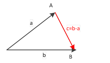
Fig. 3. Illustration of consideration vector as a point.
Let us denote the point in space Wn through P={p1, p2, …, pn}. Then, according to the method of affine space Wn is determined as follows:
 (14)
(14)
It can be written differently:
 (15)
(15)
Some point О={d01, d02, …, d0n} can be distinguished in the affine space Wn. Then its radius-vector is associated with an arbitrary point P. The affine coordinate system can be introduced into the space Wn using the concept of the radius vector, consisting of the origin - the point O and some basis of the coordinate space Kn. Affine coordinates of the point P will be the coefficients of the expansion of the radius vector in the basis
![]() (16)
(16)
An important property of space Wn is that by selecting as the point of origin О={0, …, 0} and the basis e1={1, 0, …, 0}, e2={0, 1, …, 0}, …, en={0, 0, …, 1} components of any point (ie, the elements of the tuple corresponding to it) and the coordinates of this point are the same, ie, d1=x1, d2=x2, …, dn=xn. If we select a different coordinate system, such an equation will not be satisfied.
On the basis of the affine space Wn, as well as any multidimensional affine space of affine geometry, one can easily determine other geometric space, endowed with the properties of user's interests. However, based on the space Wn it is done very simple, if the the point О={0, …, 0} and the basis e1={1, 0, …, 0}, e2={0, 1, …, 0}, …, en={0, 0, …, 1} are chosen as the coordinate system. It is easy to see that in this case the corresponding metric and topological concepts, which were discussed above, simply expressed through the points of the space Wn, or to be more precise - through their components.
In the space Wn, by analogy with other multidimensional spaces of analytic geometry, geometric shapes and operations performed on them can be put in corresponding coordinate and vector analytical description. However, the space Wn allows along with the coordinate and vector also use non-traditional descriptions. For example, the geometric shapes in space Wn can be put in correspondence with the point description. The essence of the point description is that all the points described by the figures must satisfy certain analytical relations. To specify the point description, a point P0 is allocated and then a condition is described relative to the P-P0, where P - is an arbitrary point of the described shape. For example, to describe a particular point of the space Wn, we can use the point equation:
P-P0=0, (17)
where O - zero tuple, ie, O = {0, 0, ..., 0}.
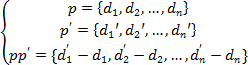
Along with the point descriptions in space Wn, a component description can also be used. The essence of the component description of geometric objects is that the components of all the points of this figure must meet certain analytical relations. The same point in space Wn can be described component system of equations:
 (18)
(18)
where di and di0, i=1, 2,…, n – components of points P and P0 respectively.
As it is seen, point descriptions are similar to traditional vector and component to coordinate. However, using the component descriptions does not require, unlike the coordinate, introducing the base into the space Wn. With regard to the point descriptions, they, unlike the vector one, can be directly used as numerical models in implementation of computer visualization algorithms of source data.
Thus, on the base of analysis of one class of multidimensional analytic geometry spaces, namely, the aggregate of the spaces that’s include the space Wn itself and spaces that may be defined based on them, one may suggests that these spaces are advantageously characterized by their simplicity and ease of use for the purposes of geometric modeling. The clarity of these spaces should be emphasized, as operating with variety of tuples of numbers is a familiar and user-friendly, especially by natural tabular interpretation of this set.
4. Conclusion
The formulated and justified higher general provisions of the rational choice of multidimensional geometric spaces for the purposes of geometric modeling have been successfully used by the authors in the development of a range of application software in the British National Centre for Computer Animation at the Bournemouth University in UK and the National Research Nuclear University in Russia. Currently, using these recommendations an interactive software tool designed for effective solution of problems of the analysis of multidimensional data by various computer visualization is being developed.
References
- Pilyugin V., Malikova E., Adzhiev V., Pasko A., Some theoretical issues of scientific visualization as a method of data analysis, Transactions on Computational Science XIX, Lecture Notes in Computer Science, Vol. 7870, Springer-Verlag, 2013, pp. 131–142.
- Matsuo Komatsu. Mnogoobrazie geometrii [The variety of geometry]. Translated from Japanese. Moscow: Science. 1981. 208 p. [In Russian]
- Efimov N.V.,Rozendorn E.R.. Linejnaja algebra i mnogomernaja geometrija [Linear algebra and multidimensional geometry]. Moscow: Science. 1970. 528 p. [In Russian]