In this article, analysis of financial and economic indexes of a number of credit organizations have been observed and picked out some different credit organizations using interactive visual interface. Data were collected from open sources, stage of processing and improvement data were considered as well as its analysis. In conducting this analysis, the so-called visual analytics paradigm has been used. For the analysis was proposed original algorithm, which was the base for developing an interactive program. Macroanalysis and microanalysis of the source data have been done. A number of judgments about the different credit organizations have been made.

Keywords: visual analysis, analysis of credit institutions, financial analysis, visual analytics.

1. Introduction

Initial table data on the considered credit organizations are multidimensional data sets with n columns and m rows, where n and m constitute several dozens and hundreds, respectively. Each row represents one of these organizations with their activity-specific parameters shown in relative columns. Derived from open sources [6], the data exhibit statistics that roots in monitoring of the organizations performed over 13 months. Such data analysis aims to provide comprehensive information on particular credit organizations or groups thereof.

This article considers proximity (similarity/dissimilarity) of separate rows (respective credit organizations), which is an area of analysts' particular interest, as well as information on certain parameters of the rows.

Within the framework of this study, the analysis was carried out by using a paradigm of the so-called visual analytics that addresses data analysis tasks through the interactive visual interface [1]. For this purpose, an original software solution has been developed to implement interactive visual analysis of multidimensional data. Based on the interactive analytical interface with visualized geometry and multidimensional table data, the solution ensures profound and easy-to-use data analysis by getting the most of human's immense potential for spatial and visual thinking [2, 3].

2. Analyzed data characteristics

As indicated above, initial data appear as multidimensional tables derived from financial statements of 938 credit organizations (Gazprombank, VTB, Deutsche Bank, etc.), with 47 parameters (net assets, net profit, personal deposits, etc.), generated over 2013 and 2014.

The tables were compiled as follows: rows represent credit organizations, columns represent parameters of the organizations. The study covers 13 months with a separate table allocated to each month. It should be noted that some data were missing, i.e. initial data were incomplete.

3. Initial data processing

Initial data processing was conducted in several stages for each of the 13 tables. The first stage embraced time interpolation of missing data, wherever possible. We used linear interpolation. If for the parameter of the jth bank and are specified, and is not specified for , then

Thus, linear interpolation helps determine some data that were not initially indicated. Fig.1 exemplifies the resulting table data effective as of June, 2014.

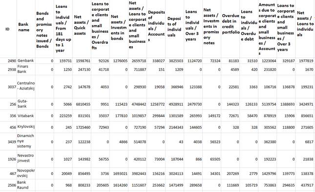
Fig. 1. An example of interpolated initial table data

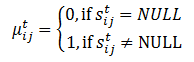
The second stage of processing and replenishment data envisaged entire elimination of initial data gaps in each of the 13 tables. For this purpose, the completeness coefficient was calculated for each credit organization.

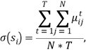
where N - the number of parameters, T- the number of time slices (tables), indicates whether the respective parameter has been specified:

If the completeness coefficient , then all the parameters (table columns) with for at least one t, are excluded from the consideration. If , then the ith credit organization is excluded from the consideration.

The third stage intended to reduce the number of credit organizations subject to further analysis. It was decided to remove all credit organizations with a zero "capital" parameter. As a result, there appeared tables with 40 columns and 81 rows.

At the fourth stage, non-integral parameters were removed from each of the 13 tables. For instance, the "net assets fixed and intangible assets", "net assets allocated to MBK" parameters were removed as they were incorporated into the "net assets" integral parameter.

The last stage of processing and replenishment data was normalization required to reduce the data to the range [0; 100].

Fig.2 exemplifies the resulting table data effective as of June, 2014.

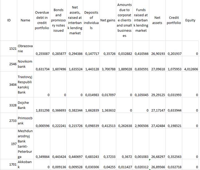
Fig. 2. Table data at the fourth stage of processing and replenishment data (fragment)

So, initial processing resulted in less size of the table data as compared to the initial data that populated 81 rows and 9 columns in each of the 13 tables. These table data became the subject of further analysis.

4. Filtered data analysis. Task formulation

As it was mentioned above, in the course of data analysis, the authors focused on similarity of certain rows (respective credit organizations) and particular parameters of similar rows. At that, we employed rows of all the 13 tables with filtered data. Let's introduce qualitative criterion of the credit organization similarity:

where - credit organizations - their parameters, ranges from 1 to 9

To address the formulated task, we resorted to the geometric interpretation. Credit organizations (table rows) were mapped to multidimensional points, organization parameters - to coordinates of these multidimensional points. In this context, similarity of credit organizations meant the Euclidean distance between points of the multidimensional space (the more the distance, the less is the similarity). In this interpretation, similarity/dissimilarity of credit organizations correlates with the distance between particular points of the n-dimensional space.

To analyze the distance between points of the n-dimensional space, we used visualization of the points. First, the initial set of points was projected to a 3D visual space. With that,

· A multidimensional point was represented as the sphere.

· If the distance between and points of the n-dimensional space appeared to be less than the pre-defined d, a cylinder was built to connect spheres and .

· The cylinder color manifested the distance between points and by color gradient from red (small distance) to dark blue (long distance).

Then the spheres and cylinders were graphically projected to the picture plane for subsequent visual analysis.

The resulting set of spheres and cylinders formed the so-called space scene with pre-determined geometry and optic (color) characteristics.

Thus, visual analysis of the space scene allowed us to assess the distance between initial multidimensional points. At the analysis stage, it was suggested that the initial value of d should be set to a large value and then be reduced to smaller values. After that, we identified sub-sets of multidimensional points with regard to the image appearing on the picture plane.

Depending on the distance between points and parameter d that changed its value in the course of the analysis, we identified the following subsets of multidimensional points:

A cluster - a subset within a given point set, where the pairwise distance does not exceed the pre-defined d value and the distance between cluster points and other points is not less than the pre-defined d value.

A remote (single) point - a point distant from all other points of the initial set more than the preset d value.

A bunch - a subset of points with most distances between points not exceeding the preset d value.

Quasi-remote (quasi-single) point - a point that is not remote but at the same time not included in a bunch or a cluster at the given grouping.

Note that the selection of bunches and quasi-remote point is carried out by man in the process of solving the aforementioned analysis problem.

5. Software solution features

To analyze distances between points of the n-dimensional space, we suggest the interactive algorithm (see the flowchart in Fig. 3).

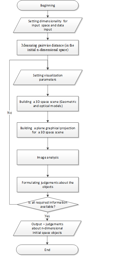
Fig.3. Interactive algorithm

The algorithm implies the analyst-computer interaction, where responsibilities are distributed as follows.

- in the course of the distance analysis, computers are used to calculate distance values, build projections and time-dependencies of coordinates;

- analysts visually perceive a projection image on the display, analyze mutual location of multidimensional points, reveal subsets and define visualization parameters.

The algorithm is implemented in the interactive software solution. Based on Autodesk 3ds Max, the solution employs the internal interpreted language maxscript. A C# library written in Visual studio 2013 was also used [4, 5].

The solution enables analysts to perform:

1. Input of initial data.

Initial data are entered only once and become available for further usage.

2. Visualization of initial data

Graphical projections are made in a standard 3ds Max window by means of a standard renderer.

3. Retrieval of point details

Point details can be viewed in a table with rows representing all displayed points and columns representing their coordinates. With that, the rows have the same background color as corresponding points to let users easily identify a subset to which a particular point belongs. Table data can be generated for any time stamp under consideration.

4. Measurement of the pairwise distance (in the initial n-dimensional space);

5. Modification of visualization parameters;

Visualization parameters include radii of spheres correlating with initial points, their color, a cylinder radius and the 3D projection space. The parameters can be modified. They are supposed to be defined at the starting point of the work.

6. Manipulations on the space scene with the use of standard 3ds Max tools. Among available tools are, for example:

а) Affine transformations of the scene;

б) Application of image filters;

в) Changes in optic characteristics of the scene;

7. Point merge into a subset

Each subset is mapped to a color that will discover the given subset during subsequent program operation.

8. Building plane graphical projections of multidimensional points

At the micro-level analysis, namely the remote point analysis, it is important to define what coordinates mostly contribute to the distance- all of them or just a few with high dissimilarity. In order to clarify this, we suggest building graphical projections of the initial subset on the plane (x_i,x_i) and view all such projections by changing the i value.

9. Creation of coordinate time-dependencies.

6. Data analysis

6.1. Macro-level analysis

In this paper, the macro-level analysis means splitting the initial point set into subsets, that ultimately aims to reveal remote point subsets. The operation algorithm assumes setting an initial d value to a large value with its further reduction, and identification of remote points.

Let's address the macro-level task for a given 81-dimensional point in a 9D space. We selected as a three-dimensional space onto which multidimensional points were projected.

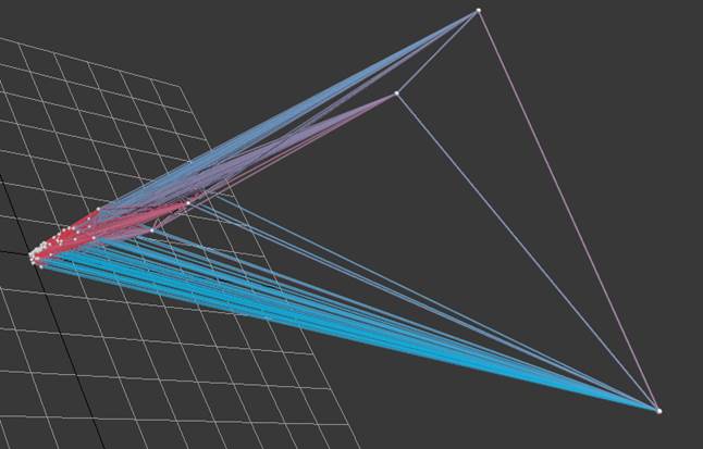
Fig.4. A graphical projection of the space scene, if

Fig. 4 illustrates a graphical projection image of the space scene, if . As it is seen, all spheres are linked to each other and, therefore, respective multidimensional points made up a cluster. This value of d will be used as the initial value to be reduced later on.

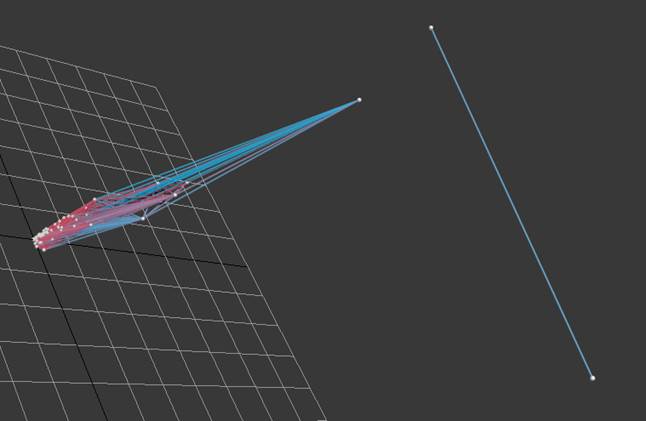
Fig.5. A graphical projection of the space scene, if

Fig. 5 demonstrates a graphical projection image of the space scene, if d=120. We can see that two spheres separated from the others and respective two multidimensional points formed the second cluster. According to the cylinder color close to bright dark-blue, the distance between these points was nearly d. We marked them dark blue.

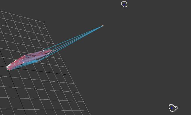
Fig. 6. A graphical projection of the space scene, if

Fig.6 shows a graphical projection image of the space scene, if . Two dark blue spheres are circled with white. Cylindrical link between them has disappeared, therefore the distance between corresponding points is greater than 100. At this d value, the points became remote. The points will not affect further macro-level analysis. Judging from the color of the cylindrical links in the remaining set, one of the points is quasi-remote and, obviously, will become remote, if d slightly changes.

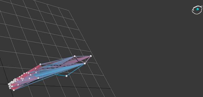
Fig.7. A graphical projection of the space scene, if

Fig. 7 illustrates a graphical projection image of the space scene, if . We marked the sphere resulting from this value of d blue (circled with white). This point will not affect subsequent splitting point sets into subsets.

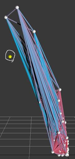
Fig.8. The graphical projection of the space scene, if

As d reduced to 60, there appeared another sphere marked yellow. Fig. 8 represents a projection image of the space scene at a given d value, the sphere is circled with white.

Likewise, further analysis will reveal successive separating spheres mapped to remote multidimensional points.

Table 1. Correlation between d and sphere colors for remote multidimensional points.

d value that triggered the change	The color of separated spheres for remote multidimensional points
34.5	Green
34	Pink
26.3	Red

Table 1 shows several subsequent values of the d parameter that entailed creation of remote multidimensional points.

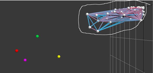
Fig.9. The graphical space scene at

Fig. 9 shows the space scene, if .

At the macro-level analysis, we revealed 7 remote multidimensional points with d ranging from 200 to 26.

At d=26 the analysis was deemed complete. However, d value could have been further reduced to reveal other remote points.

Generally, analysts should define a finite value of d with regard to available information on a particular analytical task.

6.2. Micro-level analysis

The micro-level analysis implies per coordinate comparison of remote points revealed during the macro-level analysis.

6.2.1. Plane graphic projections of multidimensional points

When building a plane graphical projection of the multidimensional point , we could assess contribution of its coordinate to the distance between this point and other multidimensional points, to learn whether it is a large value of a single or several coordinates made this point remote from the main set, or large values of all coordinates of the given multidimensional point.

Prior to drawing the projection of the multidimensional point set, the points were projected to the 3D space so as to map them to the spheres with color coding pre-determined at the stage of macro-analysis.

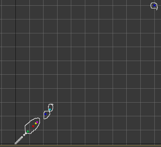
Fig. 10. The graphical projection visualizing contribution of the coordinate (written-off debt in a credit portfolio) to the distance between remote points and bunch points.

To visualize mutual location of 81 multidimensional points in the 9D space, Fig. 10 demonstrates a graphical projection to the plane for all multidimensional points, including previously revealed 7 remote points (circled with white). The projection shows that 7 spheres associated with these points stand apart from the main bunch and one of the spheres (ID=1000) is an outlier. This means that the respective coordinate contributes significantly to the distance between this multidimensional point and the other points.

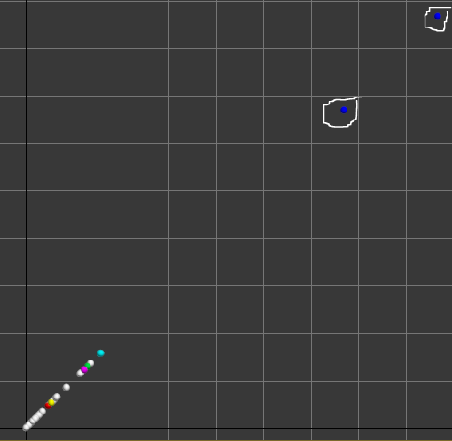
Fig. 11. The graphical projection that unveils contribution of the coordinate (net profit) to the distance between remote points and bunch points.

Fig. 11 illustrates a graphical projection of all multidimensional points to the plane . As it can be seen on the projection, for all points the coordinate does not significantly contribute to the distance, except two points visualized as two dark blue spheres (circled with white).

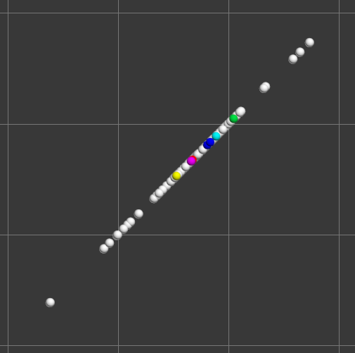
Fig. 12. The graphical projection visualizing contribution of the coordinate (net assets) to the distance between remote points and bunch points.

Fig. 12 depicts a graphical projection of all multidimensional points to the plane. On this projection, all spheres of the remote points are located in the same squares as spheres related to the main bunch points; therefore this coordinate has almost no effect on the distance between points.

6.2.2. Analysis of time dependency of multidimensional points coordinates

To analyze how point coordinates depend on time, we used standard time dependency graphs. On these graphs, the measuring unit is set to one month.

First of all, it is necessary to determine the points that should be depicted on the graph (upper left table), then select a coordinate that we want to analyze.

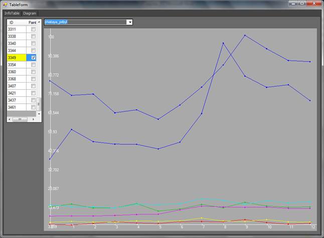
Fig. 12. The (net profit) coordinate time dependency for all remote points

Fig. 12 depicts time dependency of the coordinate for all remote points. As we can see from the graph, both dark blue points have peak values at T=7 and T=8. At peak values, coordinates increase nearly by 15-20 items (20-40%). Then the values slightly decrease.

Other points of the graph are difficult to analyze because their coordinate values are much less than those of the two dark blue points. Therefore, we built an enlarged additional graph to visualize time dependency of these two points.

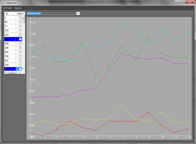
Fig. 13. Time dependency of the (net profit) coordinate for remote points with small coordinate values.

Fig. 13 shows time dependency of the coordinate for remote points with small coordinate values. Similar to the previous points, at T=7 this coordinate increases by 10-15% for all points (except the red one).

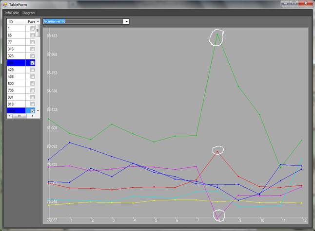
Fig. 14. Time dependency of the coordinate (net assets) for all remote points.

Fig. 14 demonstrates time dependency of the coordinate for all remote points. Red and green points spot peak values at T= while the purple point decreases the value of this coordinate.

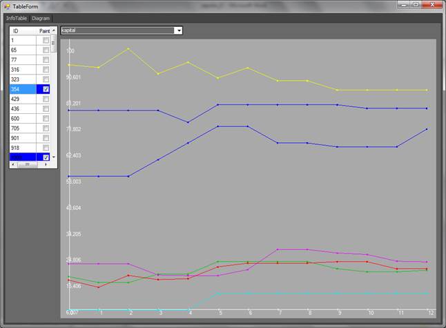
Fig. 15. Time dependency of the coordinate (capital) for all remote points

Fig. 15 shows time dependency of the coordinate for all remote points. The coordinate of the dark blue point with ID=354 changes significantly within the time interval, coordinates of the yellow point with ID=3349 show fluctuations with simultaneous decrease in values from 100 units (T=2) to 85 (T=12).

6.3. Analysis results

The analysis (both macro- and micro-levels) applied to the described example allows us to:

1. Reveal 7 remote points (dissimilar credit organizations)

Table 2. Correlation between credit organizations and remote points.

Name	ID	Color
Gazprombank	354	Dark blue
VTB	1000	Dark blue
Alfa-Bank	1326	Green
VTB 24	1623	Pink
FC Otkritie (former NOMOS-Bank)	2209	Red
Bank of Moscow	2748	Blue
Rosselkhozbank	3349	Yellow

2. Perform coordinate benchmarking of remote points (significantly different credit organizations).

Based on the benchmarking results, the following observations can be formulated:

a) Credit organizations that significantly differ from the others demonstrate dissimilarity in terms of written-off debts in their credit portfolios (fig. 10) and net profit (fig. 11), and similarity in terms of net assets (fig. 12).

b) At T=7, T=8 (i.e. the end of January and February 2014) there was an increase in the net profit (fig. 12 and fig. 13).

c) The green point (ID=1326, Alfa Bank) and the red point (ID=2209, FC Otkritie) showed dramatic growth of net assets while the pink point (ID=1623, VTB24), vice versa, indicated reduction of net assets as of T=8 (the end of February 2014) as depicted in Fig. 14.

d) Over the whole period of time, the capital remained practically unchanged for the considered points (credit organizations).

The above observations delineate preliminary results of the credit organizations analysis in a given example. Analysts could formulate more observations as to particular credit organizations, if they take into account the nature of their activities and additional task-specific information.

7. Conclusion

Hence, this paper provides analysis of multidimensional data on a number of credit organizations. The analysis was carried out by using the recent paradigm of the so-called visual analytics.

Accordingly, the original software solution has been developed to ensure interactive visual analysis of multidimensional data. The solution implements interactive geometric-visual interface with multidimensional table data, which provides an efficient and easy-to-use tool of data analysis.

First, initial data were processed (filtered) for the purposes of dimensionality reduction.

In this paper, we also addressed the macro- and micro-level analysis of filtered data and visualized the results for a certain case.

As a result, a number of preliminary observations concerning activities of the given credit organizations was formulated. It was noted that additional observations could be drawn with regard to task-specific information on the nature of credit organization activities.

References

1. Thomas J., Cook K. Cook, Illuminating the Path: Research and Development Agenda for Visual Analytics. IEEE-Press, 2005. — p. 184

2. Maslennikov O.P., Milman I.E., Safiullin A.E., Bondarev A.E., Nizametdinov Sh.U., Pilyugin V.V. Interaktivny vizualny analiz mnogomernykh dannykh [Interactive visual analysis of multidimensional data]// GraphiKon'2014: 24th International conference on computer graphics and vision: Rostov-on-Don, the SFU Academy of architecture and arts, Conference materials. - p. 51-54 (in Russian)

3. Maslennikov O.P., Milman I.E., Safiullin A.E., Bondarev A.E., Nizametdinov Sh.U., Pilyugin V.V. Razrabotka sistemy interaktivnogo vizualnogo analiza mnogomernykh dannykh [Development of a system for analyzing multidimensional data/ Scientific visualization. V.6, # 4, p. 30-49, 2014, URL: http://sv-journal.org/2014-4/089ed2.html (available as of February, 7, 2015)

4. MaxScript Help. See http://docs.autodesk.com/3DSMAX/15/ENU/MAXScript-Help/index.html (Available as of February, 7, 2015):

5. Visual C#. See https://msdn.microsoft.com/ru-ru/library/kx37x362.aspx(Available as of February, 7, 2015)

6. http://Banki.ru

7. Zagorujko N.G. Prikladnye metody analiza dannyh i znanij [Applied methods of data and knowledge analysis] – Novosibirsk, 1999. – 270 p