VISUALIZATION OF CALCULATION
OF MINIMAL AREA SURFACES
A. Klyachin, V. Klyachin, E. Grigorieva
Volgograd State University, Volgograd, Russian Federation
klyachin-aa@yandex.ru, klchnv@mail.ru, e_grigoreva@mail.ru
Contents
2. The algorithm for calculating the minimum surface
3. Visualization using the Blender environment
4. Minimal surface texturing based on the values of the Gaussian curvature
Abstract
This work is devoted to the numerical calculation and visualization of surfaces having the smallest area with a fixed boundary. The corresponding differential equation is nonlinear, so find an exact solution of the boundary value problem often is not possible. This leads to the problem of the development of effective methods for the approximate solution of the corresponding equation - the minimal surface equation. An important problem is to study mathematical methods found in terms of stability and convergence of approximate solutions. In this direction, we obtained the following results:
- We have studied some mathematical aspects of the calculation formulas and diagrams. Made some steps to justify the methods used an approximate solution of the minimal surface equation.
- On the basis of this method approximation of differential equations we obtain calculation scheme of piecewise linear surface having a minimum area of the same surfaces with a common boundary. For this calculation scheme we developed several software modules to obtain calculation results in a convenient form for subsequent processing. We done the test calculations of minimal surfaces for different spatial contours consisting of straight, parabolic and circular segments.
- The developed program is based on the library OpenGL and it allows the visualization of three-dimensional data with the ability to specify how to fill individual triangles model.
It was developed an experimental module MinSurf.py, which integrates into Blender. This module is implemented class system designed for storing models of minimal surfaces and implementation of such actions as: deformation of the surface model, automatically creating keyframes to animate the surface deformation, staining surfaces models based on technology UV-texturing.
Key words: surface of minimal area, triangulation, piecewise linear surface, approximation of the area functional, 3D modeling, deformation of surface, surface texturing.
For the design and construction of modern forms of architecture the geometric design stage occupies an important place. This is reflected in some detail, for example, in [1] and noted in the article [2], where the problem of the development of tent fabric designs is studied. Visualization and view of resulting surface is the next stage of geometric design. The problem of coordinates determining for a discrete set of points often arises in the practice of designing of complex geometric shapes coatings.
This is important for casings calculation and for control when constructing the its casings in nature. Mentioned above authors emphasize that the most preferred form of surfaces for tent fabric structures are the surface of minimal area. Such architectural structures have an attractive appearance, they are optimal in the minimum flow of materials in the construction and in the reduction of heat transfer with the environment. Visualization of such surfaces, especially with the possibility of 3D viewing, allows to make a qualitative and quantitative analysis of the constructed models, to see the distribution of physical and geometrical characteristics and values along the considered surface, to adjust of the boundary and initial data and other problems on the basis of such analysis.
Minimal surface has the smallest area compared to all other surfaces passing through the contour given in space. Intensity at each point of a minimal surface is constant. It allows to select a contour such that best efforts would experience with the transit portion of the coating [1]. To find the exact solution of the boundary value problem is often not possible. Therefore it is necessary to solve it numerically, which leads to the problem of developing effective methods for the approximate solution of the corresponding equation - the minimal surface equation. An important task is to study mathematical found methods in terms of stability and convergence of approximate solutions.
In this direction, we obtained the following results:
- We have studied some mathematical aspects of the calculation formulas and diagrams. Made We made some steps to justify the methods used an approximate solution of the minimal surface equation. [3], [4] (existence and uniqueness, convergence and stability).
- On the basis of this method approximation of differential equations approximation, the calculation scheme for piecewise linear surface (i.e. the surface, collected in the space of adjoining triangles) having a minimum area of the same surfaces with a common boundary is obtained. For this calculation scheme it we developed several software modules to obtain the calculation results in a convenient form for subsequent processing. We have done the test calculations of minimal surfaces for different spatial contours consisting of straight, parabolic and circular segments.
- We developed program that allows you to perform three-dimensional visualization of data with the ability to specify how to fill individual triangles of the model. It is assumed that the calculated data for the imaging are presented in a separate file, respectively, was done in parsing of the resulting data file and populating the corresponding arrays to store vertices, faces model were done. Suitable data structure was described. Visualization is performed by means of cross-platform OpenGL library and allows you to organize a three-dimensional overview of the model and to set the lighting parameters and parameters for the calculation of the gradient color face. Realized the The possibility to set of method of calculating the color of for each face is realized with the help of some formulas. The approach of calculating the parameters of filling separate triangle is partially implemented by approximating the Gaussian curvature of the surface.
- We developed an experimental module MinSurf.py, which integrating into environment of Blender. In this module the system of classes is implemented to store surface models and to implement such activities as: deformation of surface model, automatically to creation keyframes to animate the surface deformation, staining surfaces models based on technology UV-texturing. At the same time implement various types of deformation are implemented. In particular,
- deformation at deliberately known functions of offset vertices of the base grid,
- deformation under the influence of the phase flow, in general, non-autonomous system of ordinary differential equations,
- deformation of a simple move and rotate rotation as a solid body surface in space.
We developed also a method of storage circuits 3D model given in the form of a polyhedral surface with triangular faces. The method allows about 3 times to reduce the amount of memory required to store models. This method is based on reducing the duplication of information on the adjacent vertices of triangles.
2. The algorithm for calculating the minimum surface
Determination of the shape of a minimal surface with a given contour in a space with Cartesian coordinates  is reduced to the solution of the nonlinear differential equation
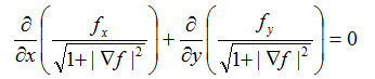 (1)
(1)
with boundary conditions of the form
 ,
,
where  is domain on the
plane
is domain on the
plane  and
and  – continuous function defined on the boundary of
this domain. Often to find the exact solution of the boundary value problem
is impossible. In this case ne, resorts to the use of numerical methods,
which leads to the problem of the development of efficient algorithms for
the approximate solutions.
– continuous function defined on the boundary of
this domain. Often to find the exact solution of the boundary value problem
is impossible. In this case ne, resorts to the use of numerical methods,
which leads to the problem of the development of efficient algorithms for
the approximate solutions.
In our work we use
the following approach involving the construction of minimal surfaces
defined over an arbitrary domain and using triangulation of the
computational domain. By triangulation we understand the following
construction. Let be given a finite set of points  on the plane. Triangulation of the set of points is a set of triangles
 satisfying the conditions
1. any point  is a vertex of at least one triangle;
2. each triangle comprises only three points from this set that are the vertices of the triangle.
Let be bounded plane domain. Triangulation of domain
is called triangulation of
arbitrary finite set of points lying in the closure  . For an arbitrary set
of values
. For an arbitrary set
of values  we define the piecewise linear function
 as follows. We construct a function on the union of all
triangles
as follows. We construct a function on the union of all
triangles  such that
  and function
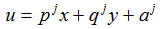 on each triangle This function is
continuous and in each triangle defined its partial derivatives
on each triangle This function is
continuous and in each triangle defined its partial derivatives
 are defined. Therefore, the area of the graph of

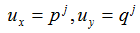
Note that the graph of a piecewise linear function is a set of triangles in a space adjacent to one another on their sides. Figures 1 and 2 show images of graphs of functions:
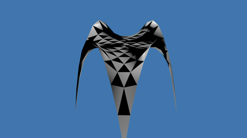
Fig. 1. Example of a piecewise linear function
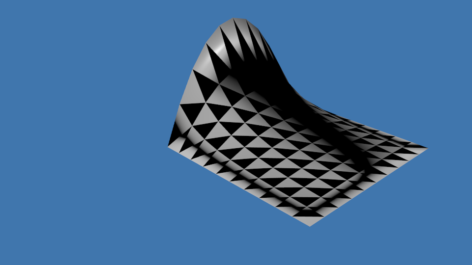
Fig. 2. Example of a piecewise linear surface
It is known that the
solution of the boundary problem for the equation (1), under certain
conditions, is equivalent to the corresponding variational problem of
minimizing the area. Therefore, finding the minimum of the function  for fixed values
  ,
corresponding to the boundary points, we obtain a piecewise-linear
surface having a minimum area of all piecewise linear surfaces with the
same boundary. Thus constructed surface and is an approximate solution
of the corresponding boundary-value problem of equation (1).
,
corresponding to the boundary points, we obtain a piecewise-linear
surface having a minimum area of all piecewise linear surfaces with the
same boundary. Thus constructed surface and is an approximate solution
of the corresponding boundary-value problem of equation (1).
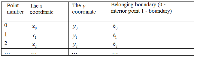
To calculate a piecewise linear minimal surface we wrote one basic procedure minimum_func() and several auxiliary procedures. Briefly we describe their work. First note that the points and triangles for considered triangulation, as well as the values of the boundary function and the calculation results are stored in four separate binary files. The structure of these files is simple. For example, the points are stored in the file points.pnt, in which the first 8 bytes are allocated to the number of points, and then each point is 20 bytes - two coordinates corresponding to the type double and membership information border (int):
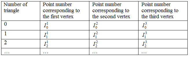
Triangulation of these points is stored in another file which has the following structure: first 8 bytes are reserved for the number of triangles, and the following data can be represented as a table
One of the supporting procedures generates a file in which for each node of the triangulation is we store a set of triangles that contain this point as a vertex. The structure of this file is as follows:
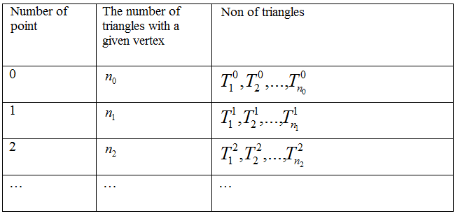
This technique will significantly reduce the time to compute
the derivatives of the variables . This is explained here as follows. Search
of function minimum is performed by gradient descent method and its application
involves an approximate calculation of its derivatives. However, when
calculating the increment of the variable functions only those triangles are
involved which contain the vertex . Thus, referring to the data of the file, we
can go through not all the triangles of the triangulation, and the
corresponding calculations are performed only for triangles is read from this
file.
Further, the results of the calculations are stored either to a binary file or a text, which can be used for further processing. For example, a call to another auxiliary function allows you to save the results of calculations in a text file format STL. The testing esting the developed program was carried out on the example of minimal surfaces such as the surface of Scherk, helicoid and catenoid. Calculation error was about 0,007-0,01% even for a small number of points (from 121 to 441 points). With the help of the developed programs were calculated minimum area surfaces for various boundary spatial contours consisting of straight, parabolic and circular sections were calculated. For building of surfaces and their imaging we have kept the results of calculations in a text file of format stl and to see it we use the program Blender 2.68a. The images for some minimal surfaces are below.
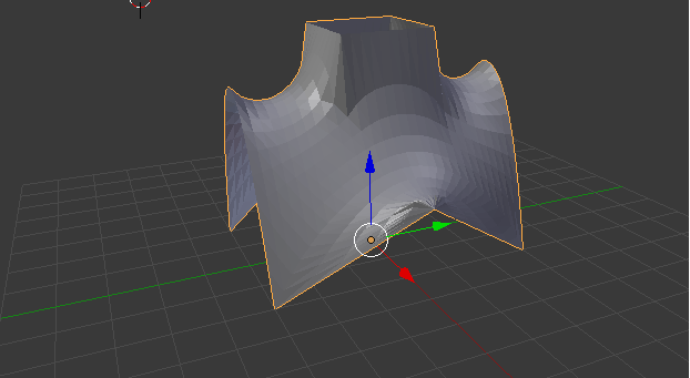
Fig. 3. Minimal surface over a hexagon with a square cut
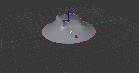
Fig. 4. Minimal surface over a circle with a square cut
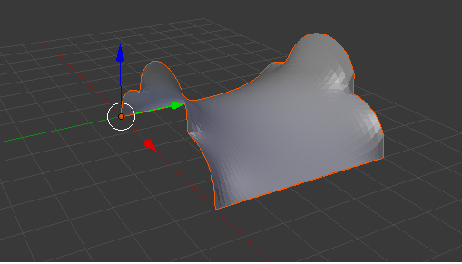
Fig. 5. Minimal surface with a boundary contour, consisting of
straight line segments and circular arcs
Figure 3 shows the surface constructed by the algorithm described above. It is stretched into two circuits. One of them consists of two parabolic arcs and four line segments projected onto the hexagon. The second circuit is a square whose projection onto the horizontal plane lies within the hexagon. Figure 4 shows the minimal surface, based on the circle and the square, located at a certain height above the plane (x,y). Figure 5 shows the surface constructed over the square and the boundary consists of two segments and six circular arcs.
Note that the approach described above allows us to find approximately the minimum surface area of a rather complicated form. For example, as noted above, Figure 3 shows a surface constructed on hexagonal domain with a square cut. Generally, to take advantage of our program, it is sufficient to have four input files that contain a list of points, triangles triangulation, information about triangles adjacent to points, and also the values of the boundary function. Thus, the advantage of the developed program is its flexibility and independence from the use of the computational grid. Moreover, the program allows you to minimize not only the area. If you need to solve the boundary value problem by a variational method for another differential equation, other than the minimal surface equation, we only need to specify the corresponding functional. However, the other software modules remain unchanged.
3. Visualization using the Blender environment
Developer environment of 3D modeling Blender [6] allows to expand opportunities due by system of plug-ins written in the programming language Python. Included module bpy [7] provides a programming interface for full control of 3D models and their properties, animation and rendering. Therefore, the proposed the environment Blender tool is very suitable for programming environment and scientific visualization. The figure below shows an environment Blender, located inside the 3D model review and placed in a special box, a text editor program designed to control the model and its properties. Consider the problem of constructing the deformed surfaces from some initial one. Visualization of successive approximations in the problem of minimizing the area functional can be reduced to this kind of problem. But when solving this problem we will put an additional condition. If the surface of 3D model is presented, we shall try to present in a universal possible form of surface deformation depending on the specific problem. For example, the deformation of the surface, its texturing, scaling, building sections, projection, etc. These problems can be represented by a single software interface and also allows you allowing to combine some surface modification in order to obtain the desired result visualization.

Fig 6. IDE Blender 2.68a
In order to implement the above-mentioned interface shows the corresponding class diagram is shown. When designing this chart, we used the ideas of object-oriented design presented in [5]. This class diagram is announced in [8].

Fig. 7. Class diagram for MinSurf.py
In this diagram, class Extent is base class for implementing various ways of visualizing models and surfaces. To modifiers and other extensions be able to convert 3D objects we need a special virtual method in the base class Object, which we call UpdateView (). Calling of this method leads, for example, to the use of a modifier Blender to the object, or to any other transformation of the visual representation of the model or surface. For example, if we want to apply the boolean modifier to the object mesh B of A, then the program is schematically as follows:
A=Mesh.new()
C=Mesh.new()
B=Boolean.new(A)
B.SetOject(B,’UNION’)
B.UpdateView().
Another possibility to solve the previous scheme is to automate the process of creating keyframe animation with object deformation. To this end, there is an additional class derives from Deformator Extent and ShapeKeys class derived from Object for storing and managing information about key forms of the object. Enabling class hierarchy Deformator extensions allow to apply the same technology as for modifiers. We give the corresponding scheme below.

Fig. 8. Class Deformator is derived class from Extent
Application of the above scheme allows to combine different imaging techniques: it we can only restrict the deformation, and also we can add the construction of the projection of the coordinate plane. In code, it looks like this.
A=Mesh.new() # Cоздается объект
B1=Deformator.new(A)# Создается объект, деформирующий А
B2=Projection.new(B1)# Создается объект осуществляющий построение проекции B1
B2.UpdateView() # Осуществляем итоговую визуализацию
This is achieved by calling UpdateView () to be decorated objects. Example of such modifiers can be found in the figures below.
Fig. 9. The plane |
Fig. 10. Deformed plane |
Fig. 11. The projection on Oxy |


Deformator class can be used for visualization in the following problems:
- variation of the surface under the action of the phase flow, in general, non-autonomous system of ordinary differential equations;
- variations of geometric characteristics of the surface when it is deformed in order to study the stability of a minimal surface;
- dynamics of changes in the shape models in the process describing the solutions of differential equations;
- process of building a system of successive approximations for the numerical solution of linear algebra problems, computational geometry, and mathematical physics.
On the following animated illustration 12 the mean curvature surface changes for Sherk surface at the local deformation is shown. Blue tone values correspond to ones close to zero, and red toness - close to the maximum of the mean curvature.

Fig. 12. Variation of the mean curvature Scherk surface
Such visualization allows you to see stress elastic shells.
4. Minimal surface texturing based on the values of the Gaussian curvature
In this section we describe the developed program for texturing surfaces on the values of a scalar function in the nodes of the base mesh. The developed program allows the visualization of three-dimensional data with the ability to specify how to fill individual triangles model. It uses a color gradient approximation method within each triangular face. It is assumed that the calculated data for visualization are presented as a separate file of format TGS, each row stores the three-dimensional coordinates of one point model.
Three successive rows define one triangle in the triangulation of the surface (see table).
| Line number in the file | x coordinate of the point | y coordinate of the point | z coordinate of the point |
| 1. First vertex of the first riangle |
0.0 | 0.0 | 3.06614 |
| 2. Second vertex of the first triangle |
0.5 | 0.0 | 1.8811 |
| 3. Third vertex of the first triangle |
0.5 | 0.5 | 1.41073 |
| 4. First vertex of the second triangle |
0.5 | 0.0 | 3.06614 |
| 5. Etc.. | 0.0 | 0.5 | 1.8811 |
In the program parsing of the resulting data file and populating the corresponding arrays to store vertices, faces model were done. Suitable data structure was described. Visualization is performed by means of cross-platform library OpenGL and allows you to organize a three-dimensional overview of the model, t0 set the lighting parameters and parameters for the calculation of the gradient color face.
The possibility of a method of calculating the color of each face was realized with the help of some formulas. The approach to the calculation of the individual parameters for the triangle shading by approximating the Gaussian curvature of the surface is implemented partially. Note that the Gaussian curvature, along with the average curvature of the surface, is one of the geometric characteristics of the surface appearing in the membrane theory of shells equations [9]. Values of the Gaussian curvature at the vertices of the surface are approximated by the formula.

where  --quantity of
the plane anglefor i-th face at the given vertex. Let us make some
clarifications. It is known that at the vertices of a polyhedral surface
Gaussian curvature is defined as the area of the spherical polygon formed by
the normals to the faces of those who own the top. This is demonstrated in the
figure below 13:
--quantity of
the plane anglefor i-th face at the given vertex. Let us make some
clarifications. It is known that at the vertices of a polyhedral surface
Gaussian curvature is defined as the area of the spherical polygon formed by
the normals to the faces of those who own the top. This is demonstrated in the
figure below 13:

Fig. 13. Calculation of the Gaussian curvature at the vertex of the polyhedron
According to the formulas of spherical geometry area of the spherical n-gon is.

where  -- interior angles of the polygon. From geometrical considerations, we have

Therefore, we finally obtain
With a view to rendering the values of this quantity the scale thresholds curvature type is constructed

and for each interval of the partition is a color from the corresponding color scale is assigned


Fig. 14.
Figure 14 shows examples of the visualization of the Gaussian curvature of minimal surfaces in four thresholds (three colors).
In this paper, the authors applied the calculation scheme for piecewise linear surface having a minimum area of the same surfaces with a common boundary. By this calculation scheme we developed several software modules that allow to obtain the calculation results in a convenient form for subsequent processing. Test calculations of minimal surfaces for different spatial contours consisting of straight, parabolic and circular sections were held. The chosen approach for the algorithms has a certain universality, in the sense that the codeof developed programs almost does not require correction when the computational domain and functional to be minimized. This makes it easy to move to modeling not only the minimal surface, but also the interface of physical media on which it reaches a minimum potential energy tension and wetting (see paras. 1.4-1.9 [10]).
This work was supported by RFBR (project № 13-01-97034 r_povolzhe_a).
[1]Mikhaylenko V.E., Kovalev S.N. Konstruirovanie form sovremennykh arkhitekturnykh sooruzheniy [Designing forms of modern architecture]. Kiev. Budivelnik, 1978, p. 138.
[2]Abdyushev A.A., Miftahutdinov I.H., Osipov, P.P. Proektirovanie nepologikh obolochek minimalnoy poverkhnosti [Design of shallow shells of minimal surface]. News KSUAE, Building construction, building, vol. 2009, no 2, 2009.
[3]Klyachin A.A. O skorosti skhodimosti posledovatelnosti, dostavlyayuschey minimum v variatsionnoy zadache [The rate of convergence of the sequence, which delivers minimum in the variational problem]. Vestn. Volgogr. Reg. Univ Ser. 1, Math. Ph., vol. 16, no 1, 2012, pp. 12-20.
[4]Klyachin A.A. On piecewise-linear almost-solutions of elliptic equations. Vestn. Volgogr. Reg. Univ Ser. 1, Math. Ph., vol. 19, no 21, 2013, pp. 19-26.
[5]E.Gamma, R.Helm, R.Johnson, D. Vlissides. Priemy obektno-orientirovannogo proektirovaniya [Priemy obektno-orientirovannogo proektirovaniya. Patterny proektirovaniya.]. Elements of reusable Object-Oriented software. St. Petersburg. Publisher Peter. 2007, p. 366.
[6]The official website for Blender Foundation. Available at: http://blender.org
[7]Official function module documentation bpy. Available at: http://www.blender.org/documentation/blender_python_api_2_64_release/
[8]V.A. Klyachin. Obektno-orientirovannaya nadstroyka dlya modulya Python upravleniya 3D modelyami v srede Blender [Object-oriented wrapper for Python module manipulate 3D models in the IDE Blender]. Materialy VI Mezhdunarodnoy zaochnoy nauchno-prakticheskoy konferentsii "Nauchnaya diskussiya: voprosy fiziki, matematiki, informatiki" [Proceedings of the VI International extramural scientific and practical conference "The scientific debate: questions of physics, mathematics, computer science"]. Moscow. "International Centre for Science and Education", 2013.
[9]I.N. Vekua. Obobschennye analiticheskie funktsii [Generalized analytic functions]. Nauka, 1988, p. 512.
[10]Finn R. Ravnovesnye kapillyarnye poverkhnosti [Equilibrium capillary surface]. Matematicheskaya teoriya [Mathematical theory]. Translate from English. Moscow. Mir, 1989, p. 312.