 .
.TOWARDS IMMERSIVE VISUALIZATION OF MATHEMATICS
A. SOURIN, O.SOURINA
Nanyang Technological University, Singapore
assourin@ntu.edu.sg
Contents
Annotation
In the modern urban society, human brain is not being sufficiently trained to deal with problems which require strong 3D spatial visualization. As a result, when teaching subjects richly infused with geometry and mathematics it is usually a challenge for the learners to follow the instructor and visualize how mathematical concepts reflect in 3D geometry and colors. We have proposed an approach that allows for defining geometry, visual appearance and tangible physical properties of virtual objects by using mathematical formulas. It allows the learners to get immersed within the 3D scene and explore the shapes which are being modeled visually and haptically. We illustrate this concept with our function-based extension of X3D and VRML. Besides definition of objects with mathematical functions straight in the scene file, standard X3D and VRML objects can be converted into tangible ones as well as augmented with function-defined visual appearances. Since the function-defined models are small in size, it is possible to perform their collaborative interactive modifications with concurrent synchronous visualization at each client computer with any required level of detail which we illustrate with an interactive modeling tool used in education in our university.
Keyworlds: immersive visualization, visual mathematics, visual and haptic rendering
In the modern urban society, human brain is not being sufficiently trained to deal with problems which require 3D perception. Everything around us is often simplified to pictures or symbols of 3D objects displayed on screens, billboards, etc. Even when commuting, we do not actually care how 3-dimensional the world around us is and how many hills and valleys our transport is crossing–it rather becomes for us just a rapid transportation from one point to another, if not to say teleportation not controlled by our brain. As a result, the brain is not being sufficiently trained to deal with problems which require 3D spatial visualization. General weakening of spatial perception and binocular vision, in particular (http://www.vision3d.com/stereo.html), has been de-facto acknowledged and reflected in education systems of different countries by making curriculum structures more geometry oriented starting from the primary or even pre-school level [3,6,9]. The importance and specifics of visualization when teaching mathematics was also discussed as a special topic at the 10th and 11th International Congresses of Mathematical Education [12, 13]. However, due to many reasons, strengthening the spatial visualization is still not emphasized as much as other competences. As a result, school children often find it difficult to deal with 3D objects, such as forming different figures of concrete 3D models, identifying the nets of solid figures and engaging in vector analysis. At the university level, there are many subjects requiring advance spatial visualization skills such as calculus, computer graphics, computer animation, geometric modeling, computer-aided design, etc. However, for the same reason as discussed above, it is often a challenge for the students to follow the instructor and visualize how mathematical concepts reflect in 3D geometry and colors.
There are a few commercially available software tools which are commonly used for doing research on mathematics and geometry as well as for learning and teaching these subjects, e.g., Mathcad (http://www.ptc.com/products/mathcad), Maple (http://www.maplesoft.com), Mathematica (http://www.wolfram.com/products/mathematica), MATLAB (http://www.mathworks.com/products/matlab), and Geometer’s Sketchpad (http://www.dynamicgeometry.com). Among other features, these tools allow learners to perform visualization of geometric shapes (2D/3D curves and surfaces) and some provide further means for making web-enabled interactive applications. However, when using these tools, the learners are only able to see images while it could be more educational to get immersed within the 3D scene and explore the shapes which are being modeled. Moreover, it would be even more beneficial if this immersion could be done collaboratively with other learners and the instructor.
There are a few examples of such collaborative approaches to learning geometry in virtual augmented worlds using VRML and on the web [1, 2, 8, 10, 13], however these projects are restricted to a limited class of geometric objects and only teach geometry rather than provide the learner with an ability to see the geometric shapes behind the mathematical formulas and illustrate how mathematics creates and supports immersive virtual spaces, as we are proposing to do in our project. Also, learning in shared virtual spaces subjects richly infused with mathematics and geometry requires for developing of interoperable data formats for exchanging mathematical objects across the Internet (e.g. project Intergeo, http://www.inter2geo.eu).
In this paper, we seek to develop an efficient way of modeling virtual objects and sharing them in cyberspace. Instead of traditionally used polygon and voxel based models, we are using relatively small mathematical functions, which define the properties of the virtual objects. We are also using haptic force-feedback so that the learners can also make physical contact with mathematically defined objects in the virtual scene, as well as with other learners. With the recent arrival on the consumer market of affordable (a few hundred dollars) interactive 3D touch devices (e.g. Novint Falcon, http://home.novint.com), haptic communication will soon become as common as interactions using mouses and joysticks. In Section 2, we discuss the visual and haptic rendering pipelines for the function-defined objects. We introduce the VRML and X3D implementation of our approach in Section 3, and give a few modeling examples in Section 4. In Section 5, we describe the interactive collaborative virtual modeling tool designed for teaching shape modeling. Finally in Conclusion we summarize the work done.
Through vision we receive most of the information about the world around us. Vision is rather a passive information collection process when we see the scene as its 2D image is projected on the retina. Touch is an active and bi-directional process of perceiving tangible properties of objects through stimulation of skin, manipulation of objects, as well as exerting forces to receive a force feedback from them. In 3D virtual environments this is done by haptic rendering using interactive force-feedback (haptic) devices. A common and relatively affordable type of these devices is a desktop robotic arm which allows for 3D navigation of a virtual tool as well as for obtaining a force feedback given in form of 3, 6 and more degrees of freedom (translation, rotation, torque). More than one device can be used by the user simultaneously. Compared to vision, very little has been done to make touch a regular part of communication with a computer, especially in shared virtual spaces.
When implemented with a computer, visual and haptic rendering pipelines originate from the virtual object definitions and end up at the visual and haptic stimuli rendered on the graphics displays and haptic devices. With the graphics displays we “sample” the visual properties of the scene while with the haptic devices we “sample” tangible physical properties of the objects in the scene. Graphics rendering gives us more information as it shows the scene all at once represented by numerous pixels constituting the image. Haptic rendering is different. It is mostly a dynamic process where we acquire and collect information about objects in form of a force feedback by moving haptic actuators on and inside the objects. The visual and haptic rendering pipelines are independent, but they are also interrelated since usually visual information is used as a guide for haptic rendering.
Since visual and touch senses are complementary and both originate from the object definitions, we propose a unified model of virtual objects where mathematical functions and procedures are used as building blocks to define geometry, as well as visual and physical properties of the objects. We will define models of objects in 3D space and time continuum, where the time is considered as yet another coordinate.
In visual rendering pipeline, at least one virtual camera is associated with the observer and each visible 3D point is displayed on a 2D image with a certain color. It requires one to define for each object its color and the components of the illumination model such as the commonly used ambient, diffuse, and specular reflections as well as transparency. Visual properties have to be associated with geometry of the object however it may be rather a placeholder or bounding surfaces, visible or invisible, for objects like clouds and fire. If functions (procedures) are used to define geometry and the components of the illumination model, we will eventually obtain a function superposition evaluating a color vector sampled by the corresponding geometry in the 3D modeling space. The geometry can be either a curve, or a surface or a solid object.
To implement haptic rendering pipeline, we need physical properties of the object which will produce forces at each point of the virtual environment that we can perceive through a haptic force-feedback device. The number of force vectors which can be calculated for any given point in 3D space depends on the haptic device used. Thus it can be one force vector for translational force or two vectors for translational and torque forces. These forces can be exerted when the user examines the outer or inner part of the object, or when the moving object collides with the haptic tool, or when a force field is produced by the object, as well as by any combination of the above. We propose to define physical properties of the virtual objects as three components: surface properties, inner density and force field. Like visual properties, the physical properties are also associated with some geometry, however it can be rather a placeholder or even an invisible container for some physical properties. To explore surface friction and density, the virtual representation of the actuator of the haptic device, which can be defined as a virtual point, vector, frame of reference or a 3D object, has to be moved by the surface or inside the object. To explore the force field, it is sufficient to simply hold the actuator within the area where the force is exerted.
We propose to define geometry of the virtual objects, as well as their visual appearance, and tangible physical properties, by concurrent using of implicit, explicit and parametric function definitions and procedures. These three components of the objects can be defined separately in their own coordinate domains and then merged together into one virtual object. We define visual appearance properties as 3D colors and geometric textures which are applied to underlying geometry. Tangible physical properties are defined as surface friction and tension, as well as inner density and forces associated with the underlying geometry. Separation of geometry and visual appearance is a common approach in different web visualization and computer graphics data formats and software libraries like VRML, X3D, Java3D, OpenGL, Open Inventor, etc. Therefore, our concept of independent definition of geometry, appearance and physics naturally can fit there. In our previous research [4, 5], we successfully implemented it with application to VRML and X3D for defining geometric objects with different visual appearances. At the present stage of our project, we expand our considerations to three components of the objects in shared virtual spaces: geometry, visual appearance, and tangible physical properties, which we define separately in their own domains by implicit, explicit or parametric functions and then merge together into one virtual object. We have published preliminary results of the project in [15] while in this paper we elaborate on the details of the visual and haptic rendering pipelines used in the VRML and X3D implementations of our modeling approach.
We define implicit functions as f(x,y,z,t)=0,
where x, y, z are Cartesian coordinates and t is the time. When
used for defining geometry, the function equals to zero for the points located
on the surface of an object. Hence, a spherical surface is defined by equation:
.
Explicit functions are defined as g=f(x,y,z,t). The function value
g computed at any point of the 3D modeling space can be used either as a
value of some physical property like density, or as an argument for other
functions (e.g., to define colors or parameters of transformations), or as an
indicator of the sampled point location. Thus, explicit functions can be used to
define bounded solid objects in the FRep sense [7]. In this case, the function
equals to zero for the points located on the surface of a shape, positive values
indicate points inside the shape, and negative values are for the points which
are outside the shape. To illustrate it, let us consider an example of function![]() which
defines a distance from the origin to any point with Cartesian coordinates (x,
y, z). If now we use function
which
defines a distance from the origin to any point with Cartesian coordinates (x,
y, z). If now we use function
![]() ,
it will define a solid origin-centered sphere with radius R. In fact this
function g=f(x, y, z) is a function of 3
variables in 4-dimensional space and it has a meaning of a distance from the
points inside the sphere to the nearest point on its surface. Without imposing
such a meaning, the equation of a solid sphere could be also written as
,
it will define a solid origin-centered sphere with radius R. In fact this
function g=f(x, y, z) is a function of 3
variables in 4-dimensional space and it has a meaning of a distance from the
points inside the sphere to the nearest point on its surface. Without imposing
such a meaning, the equation of a solid sphere could be also written as
![]() .
The original geometry of the sphere can be modified by addition of a 3D solid
texture which can be done by displacing the function values with another texture
function texture(x,y,z):
.
The original geometry of the sphere can be modified by addition of a 3D solid
texture which can be done by displacing the function values with another texture
function texture(x,y,z):
![]() . Addition
of time t to the parameters of the function would allow us to make
variable time-dependent shapes. For example, a sphere bouncing up and down by
height a during time t=[0, 1] can be defined as g = R2
− x2 − (y − asin(tp))2
− z2 ≥ 0
. Addition
of time t to the parameters of the function would allow us to make
variable time-dependent shapes. For example, a sphere bouncing up and down by
height a during time t=[0, 1] can be defined as g = R2
− x2 − (y − asin(tp))2
− z2 ≥ 0
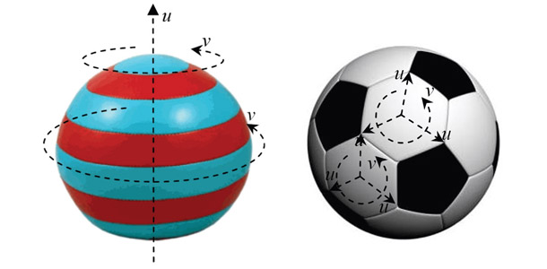
Parametric functions are, in fact, explicit functions of some parametric coordinates u, v, w and time t. They can define curves, surfaces, solid objects, vector coordinates and colors as:
x= f1(u|,v|,w|,t); y= f2(u|,v|,w|,t); z= f3(u|,v|,w|,t)
r= f1(u|,v|,w|,t); g= f2(u|,v|,w|,t); b= f3(u|,v|,w|,t)
where x, y, z are Cartesian coordinates of the points or vectors, and r, g, b are values of colors. To define a curve, only one or the u, v, and w parameters will be used, to define a surface–2 parameters are required, and to define a solid object or 3D color–3 parameters will be used. When t is added, these objects will become time-dependent. For example, the bouncing solid sphere which color changes from green to red as a function of its height could be then defined as:
x = wR cosv cosu
y = wR sinu + a sin(tp)
z = wR sinv cosu
r = sin(tp)
g = 1 - sin(tp)
b = 0
u = [0, 2p], v = [0, p], w = [0, 1], t= [0, 1]
Though we permit any combinations of implicit, explicit and parametric functions for defining the components of the shapes, only those illustrated in Figure 1 appear to have practical applications.
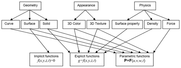
Fig. 1. Definition of geometry, appearance and physics of shapes by implicit, explicit and parametric functions.
3. Visual immersive haptic mathematics in Web3D
In our project we augment Extensible 3D (X3D, http://www.web3d.org) and its predecessor Virtual Reality Modeling Language (VRML) with function-defined objects. In X3D and VRML viewers, polygons, points and lines are used as output primitives. It requires from the extension to create output primitives and add them to the output primitives created by the viewers in their visualization pipelines [4].
Firstly, the visual rendering pipeline has to be attended. The implicit, explicit and parametric function definitions of the geometry are rendered to create output primitives which are polygons and lines in the X3D/VRML rendering pipeline. If there was any 3D texture defined for the shape by either explicit or parametric displacement of the underlying geometry, it will be taken into account at this stage as well.
Next, the color is mapped to the vertices of
the output primitives. The color can be defined either parametrically or
explicitly. When parametric functions are used, the color vector is defined as
C=F(u,v,w,t) where C=[r g b] and u,v
and w are the Cartesian coordinates of a point in 3D modeling space for
which the color is defined. When explicit functions are used, the value g
of the explicit function g=f(x,y,z,t) is mapped to color vectors
C=[r g b] by some (e.g. linear) interpolation on the given key function
values
The haptic rendering pipeline is engaged when there is a haptic device used with the application. Haptic interaction usually assumes that there is a scene being visualized that serves as a guide for the haptic device. Function parser receives coordinates of the 3D haptic contact point h=(x, y, z), three orientation angles of the haptic actuator (roll, pitch, yaw) and torque, if available. The haptic contact point is then tested whether it collides with any of the objects for which tangible properties are defined. Then, the force vectors to be applied to the haptic actuator (displacement, rotation and torque) are calculated as a result of the combined force created by the surface, density and force field properties definitions. For haptic devices with several contact points, these calculations have to be done for all of them.
Modeling of the three components of the objects—geometry, visual appearance and physical properties—can be performed either in the same coordinate system or in different coordinate domains which will then be mapped to one modeling coordinate system of the virtual object. The domains are defined by the bounding boxes (Figure 2) which specify their location and coordinate scaling. Hence, each of the components can be defined in some normalized domain and then used for making an instance of an object with different size and location. For each of the components, an individual instance transformation has to be defined. The resulting object is obtained by merging together the instances of geometry, appearance and physical properties. This approach allows us to make libraries of predefined geometries, appearances and physical properties to be used in different applications.
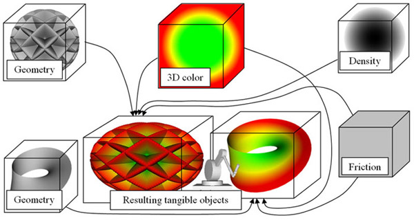
Fig. 2. Assembling geometric objects from geometry, appearance and physical properties defined in their own coordinate domains
Implementing the proposed approach in X3D and its predecessor VRML, we add new FShape and FTransform nodes. FShape node, in turn, contains FGeometry, FAppearance and FPhysics nodes. FAppearance includes
FMaterial and FTexture3D nodes. FPhysics includes FSurface, FDensity, and FForce nodes. Finally, FSurface includes FFriction and FTension nodes. FShape and FTransform nodes can be used alone as well as together with the standard X3D and VRML nodes. In the rest of the paper we will only mention X3D however VRML is supported as well.
FGeometry node is designed to define an object geometry using mathematical functions typed straight in the code as individual formulas and java-style function scripts or stored in binary libraries.
FAppearance node may contain FMaterial or the standard X3D Material nodes, as well as the standard color Texture and the function-based FTexture3D nodes. In the FMaterial node, the components of the illumination model have to be defined using functions in the same way how it can be done in FGeometry node. FTexture3D node contains a displacement function or function script for the geometry defined in FGeometry node.
FPhysics node is used for defining physical properties associated with the shape’s geometry. FPhysics contains FSurface, FDensity and FForse nodes.
FSurface node defines surface physical properties. It includes FFriction and FTension nodes. FFriction node is used for defining friction on the surface which can be examined by moving a haptic device actuator on the surface. FTension node defines the force which has to be applied to the haptic actuator to penetrate the surface of the object. The surface friction and tension are defined by explicit functions of coordinates x, y, z and the time t. Hence, the surface friction and tension can vary on different parts of the surface.
FDensity node is used for defining material density of the shape. It can be examined by moving a haptic device actuator inside the visible or invisible boundary of the shape. The density is defined by explicit functions of coordinates x, y, z and the time t, and hence it can vary within the volume of the shape. The surface of the shape can be made non-tangible, while the shape still might have density inside it to define some amorphous or liquid shapes without distinct boundaries.
FForce node is used for defining a force field associated with the geometry of the shape. The force vector at each point of the space is defined by 3 functions of its x, y, and z coordinates and the time t. The force can be felt by placing the haptic device actuator into the area where the force field is defined. Moving the actuator within the density and the force fields will produce a combined haptic effect.
FShape node may be called from FTransform node or from the standard Transform node. FTranform node defines affine transformation which can be functions of time, as well as any other operations over the function-defined shapes. These are predefined set-theoretic (Boolean) intersection, union, difference, as well as any other function-defined set-theoretic and any other operations, e.g. r-functions, shape morphing, etc.
There can be two ways of how the function-defined models of virtual objects can be used in shared virtual X3D and VRML scenes when haptic interaction is used.
First, the function-defined objects can be used within a virtual scene on their own with the geometry, appearance and physical properties defined by individual functions, scripts or procedures stored in binary libraries. In that case, all standard X3D/VRML shapes are transparent for haptic rendering even if they have common points with the function-defined shapes. Besides this, the appearance of the function-defined geometry can be declared transparent so that this invisible geometry can be used as a container for the physical properties which can be superimposed with the standard shapes. This mode can be used for modeling phenomena that can only be explored haptically (e.g. modeling wind in a virtual scene) or would require a standard X3D/VRML geometry for its visual representation (e.g. water flow can be simulated as an animated texture image with a function-defined force field associated with it). All standard shapes still will be transparent for haptic rendering even if they have common points with the invisible function-defined geometric container.
Second, besides using function-defined objects on their own, standard shapes of X3D and VRML can be turned into tangible surfaces and solid objects by associating them (grouping) with the function-defined appearance and physical properties. In that case we can significantly augment the standard X3D/VRML shapes by adding new function-defined appearance as well as allow for haptic rendering of any standard shape in the scene—features which can not be achieved by the standard shape nodes of X3D/VRML.
When haptic interaction is used, any of the objects in the virtual scene, standard or function-defined, can be used as a haptic tool avatar.
Currently, we are supporting desktop haptic devices from SensAble (Omni, Desktop and Premium 6DOF: http://www.sensable.com/products-haptic-devices.htm) and Novint Falcon (http://home.novint.com/products/novint_falcon.php). Above the device dependent layer of the haptic plug-in we have placed a common interface layer, which is a wrapper layer to handle different drivers and libraries from different vendors, and to expose a group of commonly used interfaces to the developer. By introducing this layer, we make the rest of the software device independent. The collision detection is implemented both at the level of polygons, which are obtained at the end of the X3D/VRML visualization pipeline for both standard and function-defined objects, and at the level of function definitions for the function-defined objects. The later works much faster than the polygon-based collision detection and is not restricted by the number of polygons generated in the models. When a haptic device is used to explore the virtual scene, as soon as the haptic interaction point collides with a virtual object in the scene, the whole node will immediately be sent back to the haptic plug-in. By checking the definition of the object, the plug-in will get to know whether the object is a standard object (Shape node) or a function-based object (FShape node). If the object is a standard Shape node, the plug-in will automatically switch to the polygonal collision detection mode, which we previously published in [11]. However, if the object is an FShape node, the plug-in will then get the specific collision detection mode for this FShape. If the collision mode for the FShape is specified as "polygonal", the plug-in will perform collision detection with the polygons generated from the FGeometry function definition. If the collision mode is specified as "function", the function definition of FGeometry will be directly retrieved within the plug-in and used for computing of the collision detection based on the function values rather than on polygons [15].
4. Examples of modeling with functions
Let’s consider a few examples. To ease reading and save space, the codes of the examples are written using VRML-style encoding however XML encoding for X3D can be used as well.
Examples of function definitions of two spheres, as it was discussed in Section 2, are given in Figure 3. In Figure 3a, the sphere is defined by an explicit FRep function with a solid texture defined as a displacement noise function and a color defined by 3 parametric functions. In Figure 3b, a parametrically defined sphere bounces up and down with its color changing as a function of height and time.
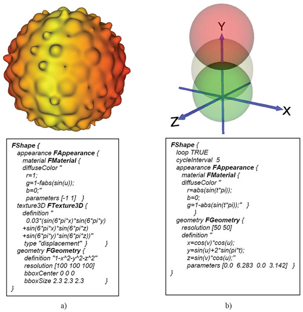
Fig. 3. Examples of function definitions in the extended VRML code. a) A solid textured sphere is defined by explicit FRep functions. b) A bouncing sphere with a time-dependent color is defined parametrically.
In Fig. 5, an example of modeling a tangible “watermelon” is given. The geometry, appearance and physical properties of this object are defined with explicit FRep functions [7]. The geometry is defined as a sphere with a piece cut away from it by a semi-infinite solid object defined by 3 planes:
func = ( 1 − x2 − y2 − z2 ) & (−(( z − x )& y & z )) ≥ 0
where the set-theoretic intersection is denoted as &. The set-theoretic operations (STO) are implemented in the extension both by min/max and r-functions [7]. It is up to the user to decide which continuity of the resulting function is required to select the STO implementation to be used. The fastest but C(0) continuity is produced by the provided min/max function implementation while any other continuity C(n) can be achieved by using r-function implementation of STO, which is also supported by the software.
The color is then represented by a 3D color field defined in the same geometric coordinate space. The function of this field is defined as a distance from the origin
![]()
with distortions defined by a specially designed noise function
noise = 0.01( sin(12atan( x, z + 0.04sin(25y))) − 0.7).
The function values are then linearly mapped to the color values according to a designed color map. The uneven shape of the color iso-surfaces was used for making green patterns on the surface of the “watermelon”. This was achieved by mapping the respective function values from 0.98 to 1 to RGB values of colors ranging from [0 1 0] to [0 0.2 0]. The colors inside the watermelon are also created by linear mapping of the respective color function values to different grades from yellow, through white, and finally to red colors.
The density inside the watermelon is defined as a distance function script with a value 0.8 near the surface and a variable value g inside it:
g = 0.3 + 0.2sin(120px)sin(120py)sin(120pz)
In Figure 4, the density values are displayed with different colors and intensities. The zoomed section of the inner part shows how the density changes to simulate a crunchy body of the watermelon. The surface friction and tension are constant 0.1 and 1, respectively. The whole FShape object definition code is built by putting together the four fragments of the code given in Figure 4.
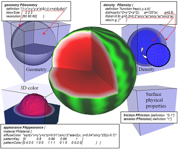
Fig. 4. Modeling “watermelon” by assembling the object from geometry, appearance, and tangible surface properties and inner density.
In Figure 5, we make a scene from standard and function-defined shapes. The fan is made from standard polygonal VRML objects. It is defined as a touch sensor so that when it is clicked its blades will start rotating. The surfaces of the standard objects—fan, cabinet and carpet—are made tangible by grouping them with a function defined object which has only a tangible surface property defined. A function defined air-flow is defined within a transparent geometric cone which is attached to the fan blades, as displayed in the figure. The surface of the cone, which is defined by parametric functions, is used for triggering collision detection. When the fan starts blowing, the force field will be activated as well, and it can be felt with a haptic device when its virtual contact point is placed inside the invisible cone. In this example, we also illustrate how different properties can be modeled in different coordinate domains and then mapped into one object. Hence, the force field is originally defined in a unit bounding box which is then mapped to the bounding box defined for the geometric container, which is the cone.
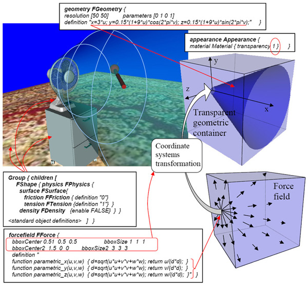
Fig. 5. Making tangible wind in a shared virtual scene.
Another example of defining tangible objects in X3D scene is given in Figure 6. Here, an X3D model of a moving shark, which is linked (inlined) from the companion web resource for the X3D reference book (http://x3dgraphics.com), is turned into a tangible solid object by associating (grouping) it with the function-defined physical properties which are set as a medium-tension surface with friction and non-uniform density inside it (softer at the peripheral parts and harder when closer to the shark’s backbone). Besides this, a time-controlled force field is defined around the shark’s tale. The force vector follows the motion of the tale which is defined within a cycle interval of 5 sec. To feel this force, the haptic actuator has to be placed inside an invisible geometric container which is a box defined by FRep functions as an intersection of 6 half-spaces bounded by planes. The box’s appearance is defined as invisible to the viewer (transparency 1). The force vectors are defined by parametric functions for each point inside the box defined by their Cartesian coordinates (u, v, w) and time t. Infinitely repeating 5 sec time intervals (cycleInterval 5) in the virtual scene map to time intervals [0, 1] within the parametric definitions of the force vector (timeSpan 0 1). Since the time in the scene is controlled by the computer timer and the same time interval is used both for the force and in the model definition of the shark, the motion of the tail will be synchronized with the forces simulating water pressure created on the sides of the tale when it waves. The magnitude of the force vector increases for the points closer to the end of the tale and decreases with increasing the distance from it. For illustration purposes, the box and the force vectors are shown in the figure as a transparent blue box and black arrows, respectively.
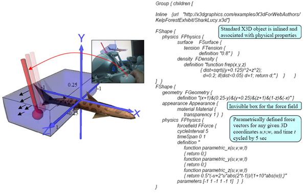
Fig. 6. Adding tangible physical properties to X3D scene.
5. Practical application example
In this Section we illustrate how mathematical functions can help solving a problem of compression of large polygon meshes. Complex geometric shapes are often represented as large polygon meshes which have a fixed Level of Detail (LOD) and require a considerable amount of memory for their handling. It is therefore problematic to use these shapes in 3D shared virtual spaces due to the Internet bandwidth limitation. To address this problem, polygon meshes can be replaced with models obtained from the use of Partial Differential Equations (PDEs) generally represented by relatively small sets of PDE coefficients [16]. Mathematically, given a 3D geometric shape s defined by vertices P = {piÎR3 | 1≤ i ≤ Mp} on its surface, a 3D geometric shape S, which is a close parametric approximation of the shape s, can be derived. The shape S is defined by a group of PDEs which are parametric functions for Cartesian coordinates x, y, z with Mc coefficients such that Mc << Mp.
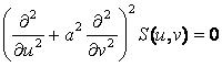
Bloor et al [17] pioneered the research on using PDEs in computer graphics by producing a parametric surface S(u, v) defined as a solution to an elliptic fourth order PDE:
(1)
where a ≥ 1 is a parameter that controls the relative rates of smoothing between the u and v parameter directions. The partial differential operator in Equation (1) represents a smoothing process in which the value of the function at any point on the surface can be understood as a weighted average of the surrounding values. Thus, a single PDE patch of a surface is obtained as a smooth transition between the boundary conditions. Commonly, the PDE boundary curves are extracted in a circular though not necessarily co-planar way around the object so that the whole reconstructed object is a single entity in its parametric space, and that each PDE patch is adjacent to maximum two other patches (See Fig. 7a). In the patchwise PDE method proposed in [16], each shape is represented by patches with their own parametric coordinate systems (Fig. 7b). This configuration allows for representing shapes with branches and for preservation of irregular and sharp details on the object surface by matching the respective patches with various sizes and orientations to the surface.
(a) (b)
Each PDE patch P(u, v) can be formulated by Equation (1). Assuming that the effective region in the uv space is restricted to 0 ≤ u ≤ 1 and 0 ≤ v ≤ 2π, and using the method of separation of variables, the analytic solution to Equation (1) is generally given by
![]() (2)
(2)
![]() (3)
(3)
![]() (4)
(4)
![]() (5)
(5)
and vector-valued PDE coefficients α00, α01, …, αn3, αn4 and β11, β12,…, βn3, βn4 are determined by the boundary conditions. In Equation (3), A0(u) takes the form of a cubic polynomial curve with respect to u. In Equation (2), the term A0(u) is regarded as the “spine” of the surface, while the remaining terms represent a summation of “radius” vectors that give the position of P(u, v) relative to the “spine”. Therefore, the PDE surface patch P(u, v) may be pictured as a sum of the “spine” vector A0(u), a primary “radius” vector A1(u)cos(v) + B1(u)sin(v), a secondary “radius” vector A2(u)cos(2v) + B2(u)sin(2v) attached to the end of the primary “radius”, and so on. The amplitude of the “radius” term decays as the frequency increases. It can be observed that the first few “radii” contain the most essential geometric information while the remaining ones can be neglected. Therefore, Equation (2) can be re-written as:
![]() (6)
(6)
where only N “radii” are selected and the number of vector-valued PDE coefficients is Mc=4´(2N+1). Strictly speaking, this equation needs a remainder term to guarantee that the boundary conditions are satisfied. The boundary conditions imposed on Equation (6) take the following forms:
P(0, v) = C0(v)
P(u1, v) = C1(v) (7)P(u2, v) = C2(v)
P(1, v) = C3(v)
where C0, C1, C2 and C3 are isoparm boundary curves on the surface patch at u = 0, u1, u2, and u = 1, respectively, and 0<u1, u2<1. Fig. 8 illustrates the layout of the PDE boundary curves for an individual PDE patch, where C0 degenerates into one point.
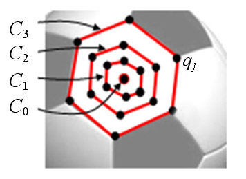
Fig. 8. Boundary curves for an individual PDE patch.
Theoretically, such a PDE patch can be of any shape provided:
· It can be mapped from a planar u,v domain to the 3D surface;
· The points which define its border lay on the surface of the object; and
· The patches can be blended together seamlessly.
More details about blending and rendering of the patches can be found in [16] while [18] proposes how to automatically reconstruct PDE boundary curves from any given large polygon mesh.
The described PDE compression method is implemented as a part of the function-based extension plug-in to VRML and X3D [15, 17, 18]. The automatic curve extraction software is a standalone program which has to run first. It reads polygon mesh data (e.g. in the commonly used .OBJ data format) and creates data with the coordinates of the boundary curves. The user can only define the degree of representation which will result in various numbers of the boundary curves derived. These curve serve as an input data for the PDE shape defined in VRML/X3D and they can be either located on a client computer or on a web server. When the VRML/X3D code is run, it first detects whether the PDE plug-in is installed. If the plug-in is installed, it will process the PDE shape definition given by the PDE curves file name and a few rendering parameters. The PDE plug-in software is implemented as two binary DLL library functions. The first one will be called by the VRML/X3D viewer only once to read the PDE curve data and to calculate the PDE coefficients. The calculation time depends on the number of the PDE curves read and in many cases is performed at interactive rates. After the PDE coefficients are calculated, they are stored in a file on the hard drive which will be read by another DLL function that will perform rendering of the PDE shape. This function calculates the polygons interpolating the PDE shape and sends them into the VRML/X3D rendering pipeline making the PDE shape a legitimate part of the shared virtual scene that can be further treated as any other standard VRML/X3D shapes. In Fig. 9 the VRML shapes reconstructed from the original polygon meshes are displayed. The Stanford Bunny mesh has a size of 539 Kb while the derived coefficients file is only 86 Kb and 120 Kb for 180 and 250 PDE patches, respectively. In Fig. 10 two PDE shapes are displayed in a VRML environment.

Fig. 9. Reconstructions of Stanford Bunny from 180 and 250 PDE patches.
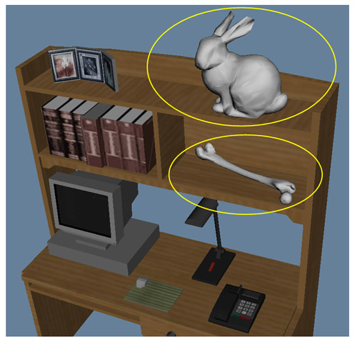
Fig. 10. PDE shapes (highlighted) placed in a VRML environment.
6. Visual mathematics in education
Since writing meaningful mathematical function and scripts can be a challenge, especially when there is a need to obtain 3D coordinates of the objects in the virtual scene, we have developed a shared virtual tool where the users are able to collaboratively model complex 3D shapes by defining their geometry, appearance and physical properties using analytical implicit, explicit and parametric functions and scripts (Figure 11). The tool visualizes the language of mathematics in forms of point clouds, curves, surfaces and solid objects. The users may go inside the 3D scene being modeled and explore it by walking through it, as well as haptically investigate it.
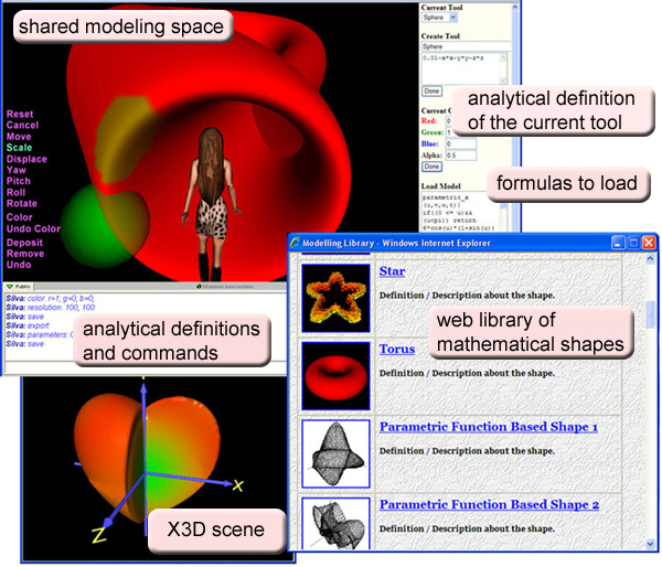
The tool is not intended for making hi-end geometric models, such as those that can be created with CAD tools like Maya and 3D Studio MAX. Instead it rather emphasizes the modeling process itself by demonstrating how complex geometry, appearance and physical properties can be defined by small mathematical formulas. The users select from the predefined sets initial shape, tools, geometric and appearance operations or define them analytically which makes the tool open to any customization. Models defined by analytical formulas or function scripts can be easily modified on-the-fly in the virtual scene either by editing the formulas or by doing iterative interactive modifications. To apply a virtual tool, the user clicks at any point on the object being modeled. The 3D object representing the current tool will be placed to the scene at the selected point. The size, position and orientation of the tool can be changed interactively either with the haptic device or with a common mouse. After placing the tool, the user selects one of the pre-defined operations to modify the geometry or the color of the object. In the screen shot which is shown in Figure 7, three such operations are defined: removing of material, depositing of material and applying color. Removing material subtracts the object representing the tool from the current object. Depositing material unifies the tool with the current object. Coloring operation blends the color assigned to the tool with the current 3D color of the object according to the transparency assigned to the tool. The color blending is performed only at the part of the current object that intersects with the tool. When the tool is not transparent, the color of the tool overrides the color of the current object at the application area. There is also a set of commands, which the learners can type in the chat box of the browser and immediately see how the shape changes. The software filters out the shape-modeling commands from other chat messages and processes them accordingly. The function description of the current shape can be generated and saved for future use on their own or within X3d or VRML virtual scenes.
The tool is developed as a server-client application. The shared collaboration when using this tool is achieved by exchanging models of the virtual objects between the clients. Since the size of the function-defined models is small, it can easily be done. The server is only used for broadcasting messages with models and commands to all the participating clients.
To avoid making simultaneous changes to the model by several clients, we employ a locking mechanism. The lock is activated and released automatically when the client wants to modify the scene. If the lock is already obtained by another client, the modification is ignored.
Since the function-defined models are small in size, the whole model is transmitted between the clients to support synchronized visualization of the changes being done to it. Besides the shared version, we have also developed a web-enabled individual version. With haptic plug-in installed, the tools allow the users to define physical properties of virtual objects and their haptic rendering with force-feedback devices as well.
The developed software is used in collaborative work when teaching students of the School of Computer Engineering in Nanyang Technological University in Singapore as a part of the computer graphics assignment “Implicit Fantasies and Parametric Metamorphoses in Cyberworlds”. The students are asked to create virtual scenes with objects defined by implicit, explicit and parametric functions. The objects must be created with set-theoretic operations from simple building blocks defined by functions straight in the scene code or using the interactive tool described in Section 5. The objects must have continuous level of detail, which can naturally be provided by using different resolution parameters in the function definitions for different distances to the observer. The objects must also be developed with morphing and animation transformations, also defined by mathematical functions. An example of a function-based definition of a virtual clock showing the actual time is given in Figure 12. Here, time-dependent transformations are used for moving the clock hands so that they follow the actual time which is synchronized by obtaining the timer events from the computer clock. In the mathematical formulas, the time variable t increments from 0 to 1 while this range maps to the actual time used in the scene within each node in a field cycleInterval. Hence, the second hand makes one full 2p rotation for 60 seconds, minute hand – for 60×60=3,600 seconds, and hour hand for 12×60×60=43,200 seconds. The rotation angle of the hour hand is adjusted by the hour zone of Singapore, which is GMT-8 hours: 2p×(8/12). The geometric objects used in the scene and their color are defined by parametric functions.
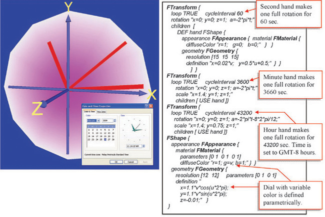
Fig. 12. An example of making a virtual clock by parametric functions and time-dependent affine transformations.
This assignment immerses the students into the world of mathematical definitions and teaches them how to see geometry, motions and colors behind mathematical formulas. A few examples of what the students are able to achieve after only 5 lab sessions are given in Figure 13. A short video illustrating some of the experiments with the developed software as well as a quick look at the student lab is available at http://www3.ntu.edu.sg/home/assourin/Fvrml/video.htm.
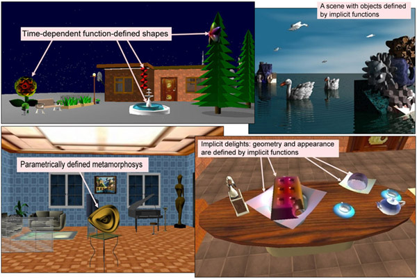
Fig. 13. A virtual scene where all objects are defined by implicit functions.
Conclusion
We have developed a function-based approach to web visualization where relatively small mathematical formulas are used for defining the object’s geometry, appearance and physical properties. It allows the user to get immersed within the 3D scene and explore the shapes which are being modeled visually and haptically. To illustrate this concept, we developed a function-based extension of X3D and VRML. With this extension, we are able to provide haptic feedback from both standard objects of X3D/VRML, as well as from advanced 3D solid objects and force fields defined by mathematical functions and procedures. We have designed and developed an innovative application for collaborative teaching of subjects requiring strong 3D geometric interpretations of the theoretical issues, which, in turn, caters to the diverse needs of learners and has the space for continuous improvement and expansion. Our software unifies, under one roof, and provides learners with the ability to: /1/ interactively visualize geometry and appearance defined by analytical formulas, /2/ perform a walkthrough the created scene, as well as haptically explore it, and /3/ make the scene a part of any other shared virtual scene defined by X3D and VRML. As well our tool puts the emphasis on the modeling process itself by demonstrating how geometry, appearance and physical properties can be defined by mathematical formulas. Another benefit is that the software does not require purchasing any licenses and is available anytime anywhere on any Internet-connected computer.
Acknowledgements
This project is supported by the Singapore Ministry of Education Teaching Excellence Fund Grant “Cyber-learning with Cyber-instructors” and by the Singapore National Research Foundation Interactive Digital Media R&D Program, under research Grant NRF2008IDM-IDM004-002 “Visual and Haptic Rendering in Co-Space”.
1. Guimarães, L.C., Barbastefano, R.G., Belfort, E. Tools for teaching mathematics: A case for Java and VRML, Computer Applications in Engineering Education, 8(3-4), 157-161, 2000
2. Kaufmann, H., Schmalstieg, D. Designing Immersive Virtual Reality for Geometry Education. IEEE Virtual Reality Conference, VR 2006, pp. 51-58. IEEE CS Press (2006)
3. Kunimune, S., Nagasaki E. Curriculum Changes on Lower Secondary School Mathematics of Japan - Focused on Geometry. 8th International Congress on Mathematical Education. Retrieved January 8, 2008, from http://www.fi.uu.nl/en/Icme-8/WG13_6.html (1996)
4. Liu, Q., Sourin, A. Function-based shape modelling extension of the Virtual Reality Modelling Language. Computers & Graphics, 30(4), 629-645 (2006)
5. Liu, Q., Sourin, A. Function-defined Shape Metamorphoses in Visual Cyberworlds. The Visual Computer, 22(12), 977-990 (2006)
6. Mathematics Syllabus Primary. Ministry of Education Singapore. Retrieved from http://www.moe.gov.sg/education/syllabuses/sciences//maths-primary-2007.pdf (2009)
7. Pasko, A., Adzhiev, V., Sourin, A., Savchenko, V. Function Representation in Geometric Modeling: Concepts, Implementations and Applications. The Visual Computer, 11(8), 429-446 (1995)
8. Pasqualotti, A., Dal Sasso Freitas, C.M. MAT3D: A Virtual Reality Modeling Language Environment for the Teaching and Learning of Mathematics. CyberPsychology & Behavior, 5(5), 409-422 (2002)
9. Secondary Mathematics Syllabuses. Ministry of Education Singapore. Retrieved from http://www.moe.gov.sg/education/syllabuses/sciences//maths-secondary.pdf (2009)
10. Song, K.S., Lee, W.Y. A virtual reality application for geometry classes. Journal of Computer Assisted Learning, 18, 149-156 (2002)
11. Sourin A, Wei L. Visual Immersive Haptic Rendering on the Web. 7th ACM SIGGRAPH International Conference on Virtual-Reality Continuum and its Applications in Industry, VRCAI 2008, 8-9 December (2008)
12. TSG 16: Visualisation in the teaching and learning of mathematics, 10th International Congress of Mathematical Education. July 4-11, 2004, Copenhagen, Denmark, from http://www.icme-organisers.dk/tsg16 (2004)
13. TSG 20: Visualization in the teaching and learning of mathematics, 11th International Congress of Mathematical Education. July 6-13, 2008, Monterrey, Mexico, from http://tsg.icme11.org/tsg/show/21 (2008)
14. Yeh, A., Nason, R. VRMath: A 3D Microworld for Learning 3D Geometry. In L. Cantoni & C. McLoughlin (Eds.), Proceedings of World Conference on Educational Multimedia, Hypermedia and Telecommunications 2004, pp. 2183-2194, Chesapeake, VA: AACE (2004).
15. Wei, L., Sourin, A., Sourina, O. Function-based visualization and haptic rendering in shared virtual spaces. The Visual Computer, 24(5):871-880 (2008)
16. Y. Sheng, A. Sourin, G. González Castro, H. Ugail, “A PDE Method for Patchwise Approximation of Large Polygon Meshes”, The Visual Computer, 26(6-8), 975-984 (2010).
17. M. Bloor, M. Wilson, “Generating blend surface using partial differential equations”, Computer Aided Design, 21(3), pp. 165-171,(1989).
18. Ming-Yong Pang, Yun Sheng, Alexei Sourin, Gabriela González Castro, Hassan Ugail. Automatic Reconstruction and Web Visualization of Complex PDE Shapes. 2010 International conference on cyberworlds. IEEE CS Press, Accepted. Singapore, 20-22 October, (2010).